Eddy current decay in the SPS main dipoles

Overview

Most beams injected into the SPS sees a drift of the orbit during the injection plateau when uncorrected. This is due to decaying eddy currents causing a dipole fields, which are primarily caused by ramp-down of the main dipoles on the previous cycle, but could also be mixed with effects from the ramp-up if the flat-top is short. Therefore, cycles that see the largest effects on the beam caused by eddy currents are ones that inject the earliest. In the SPS, this is the fixed target cycle, which 200 ms after cycle start at 14 GeV. For the main dipoles this is equivalent to a main dipole field around 0.0622 T, or 161 A, compared to the idle current 155.53 A, or 0.0603 T.

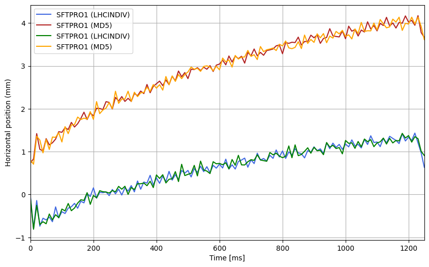
Normally the SFTPRO cycle has a momentum ramp at injection to counter the eddy current decay from the ramp-down of the MD1. However after flattening the momentum ramp, and thus isolating the decaying effects we can see the orbit decay clearly on the beam orbits, here measured during BC MD 2025-03-18 , with different preceding cycles, either an LHCINDIV, which has ramped down from 450 GeV, or an MD5, which has an identical ramp-down to the MD1 from 200 GeV:

Modeling current decay

The original intention was to use magnetic field measurements to capture eddy current decay in the main dipole fields, however it has been shown through different measurements in the main dipoles in the 867 measurement lab, on the B-Train, and on the beam that the dynamic effects are not consistent through all scenarios. Specifically the lab measurements of a single MBA magnet shows decaying effects in the order of tens of milliseconds, whereas the B-Train measurements sees decays taking hundreds of milliseconds, and finally on the beam the decays can take several seconds to decay completely.

This inconsistency between different measurement systems, and negligible effects on the lab measurements, suggest that the main dipole itself sees few little eddy currents propagating through the magnet yoke, but it is rather an effect on the vacuum chamber, as the SPS B-Train consists of an MBA and an [[SPS Main Dipoles|#MBB]] measured in series, which in turn has 2 vacuum chambers connected together.

Decay constant in the main dipoles

Field decay on B-Train measurements

For the SPS main dipoles we can find the Eddy current decay constant by looking at the ZERO cycle for idle current, SFTPRO1 flat top, even when the flat top is ramping slightly.

Second analysis

We use a dataset with 3x ZEROs after SFTPRO1 ramp down, and to compensate for drift in the acqusition of the ZERO cycles, we add an additional linear component to the curve fit and achieve the following:

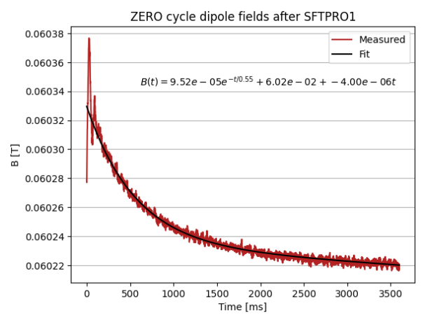
We see that the fit improves to the previously fitted decay constant. Here we instead see a decay constant of $\tau =550ms$, however this still differs greatly from effects seen on the beam during Eddy current decay constant.

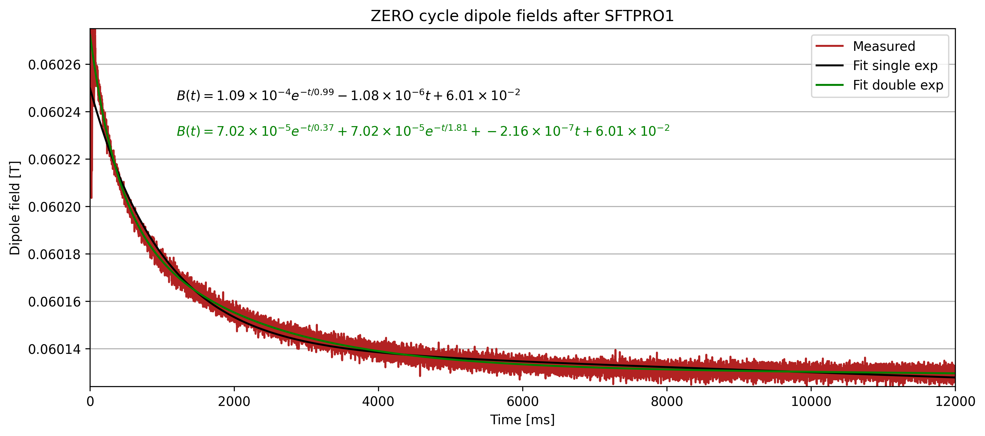
The fit with 10x ZEROs fit better than with 3x ZEROs, primarily with the added information of longer decay. Note that we don’t include the first 120 points/ms in the fit, as the power converters still has significant ripples at that time.

Effectively the time constant increases from $\tau =550ms$ to $\tau =1000ms$ for the single exponential, while for the double exponential the time constants change slightly.

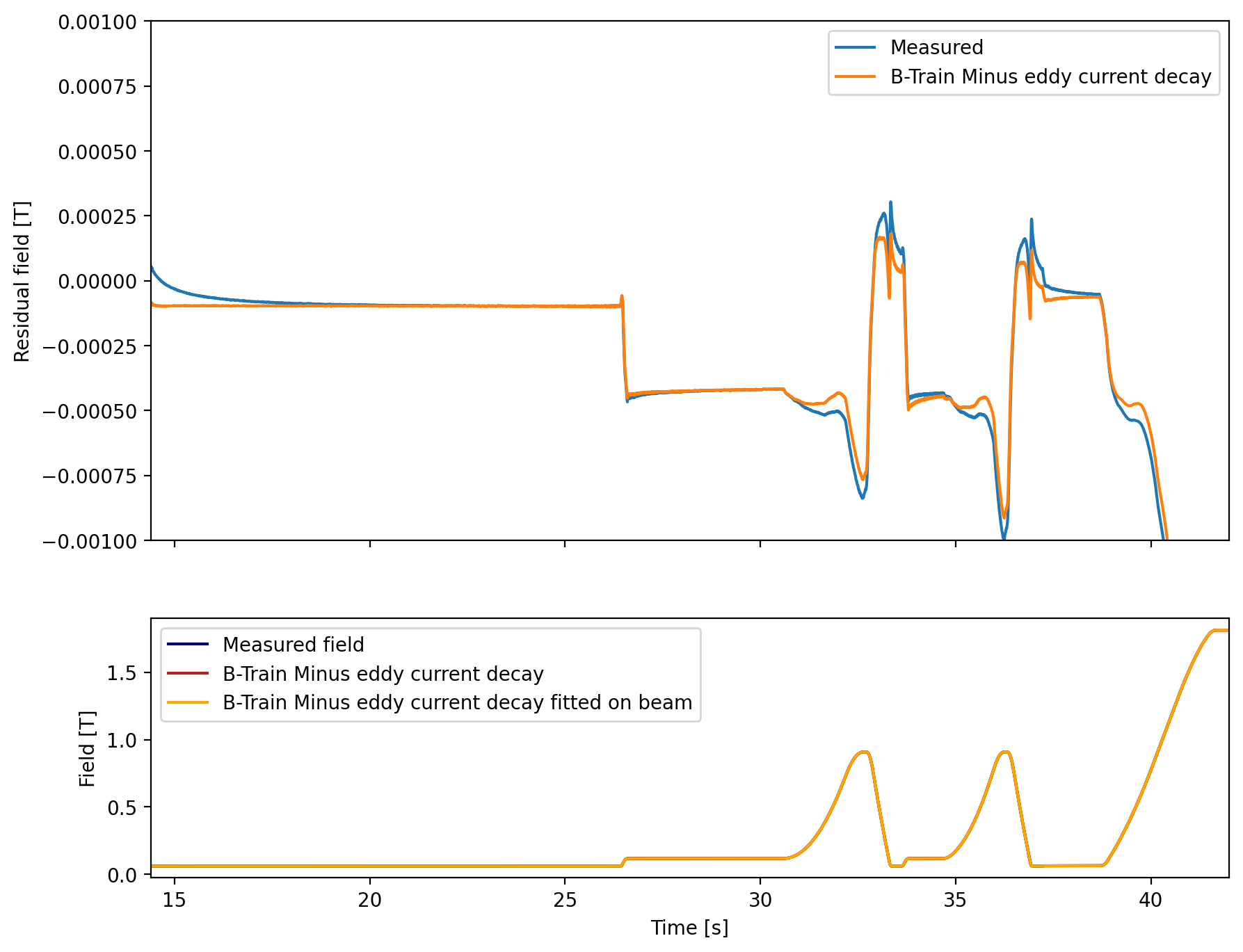
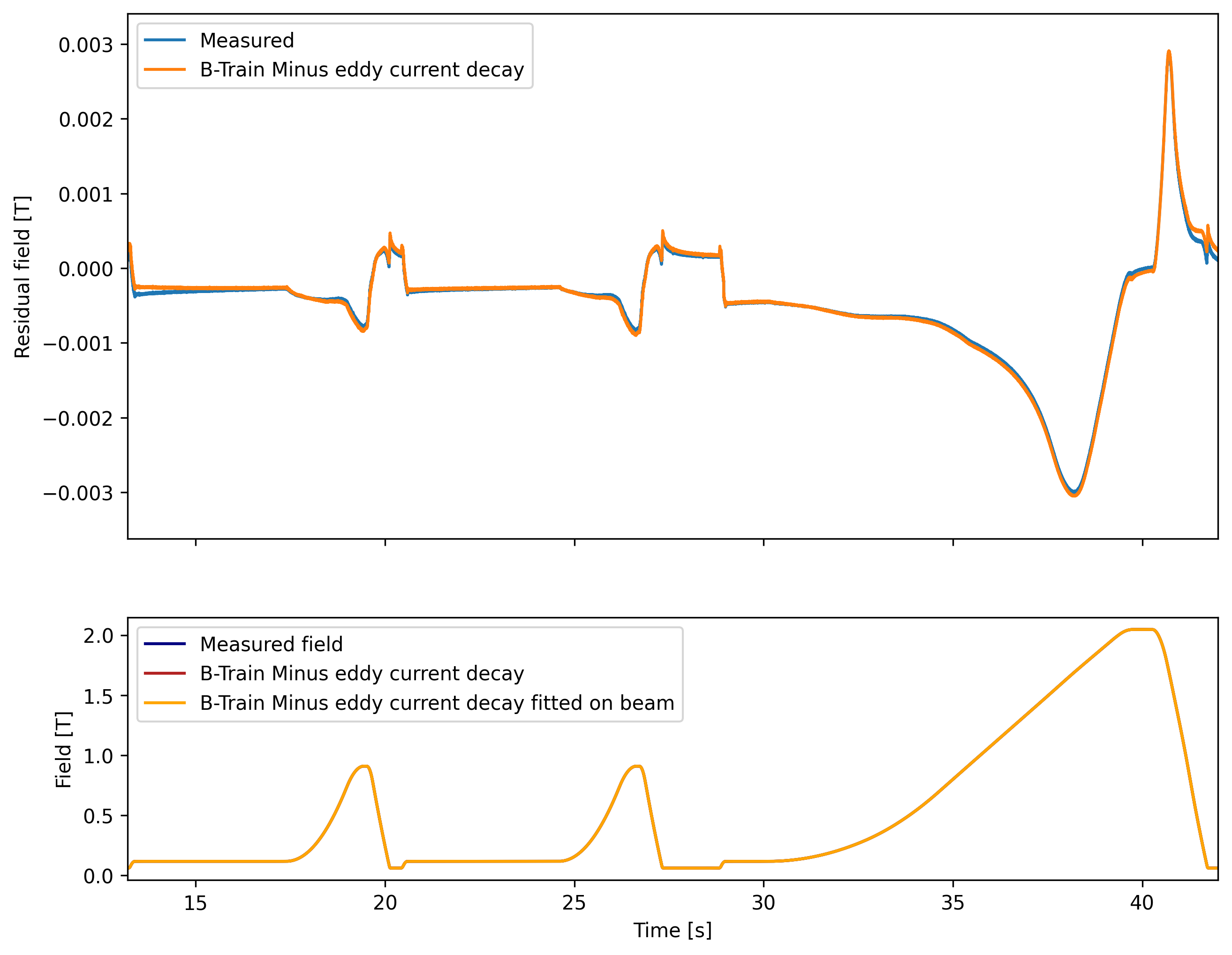
Eddy current decay parameters: -1.01e-07, 0.37 s, -2.41e-08, 1.86 s

Third approach

We use another dataset to crosscheck

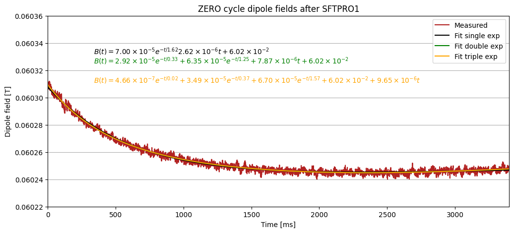
We are drifting upwards, and we ignore the ripple in the beginning of the ZERO cycles.

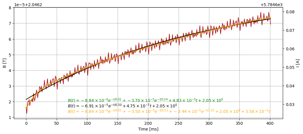We choose the time constants from the ZERO cycle decays due to the additional points available for fitting (3000 vs 400).

So ${\tau }_1=20$ ms, ${\tau }_2=370$ ms, ${\tau }_3=1.57$ s. Based on these time constants, we fit the exponential convolution coefficients to be $C_1=3.98\times 10^{-7},C_2=-1.23\times 10^{-7},C_3=-5.41\times 10^{-9}$ on a flat part.

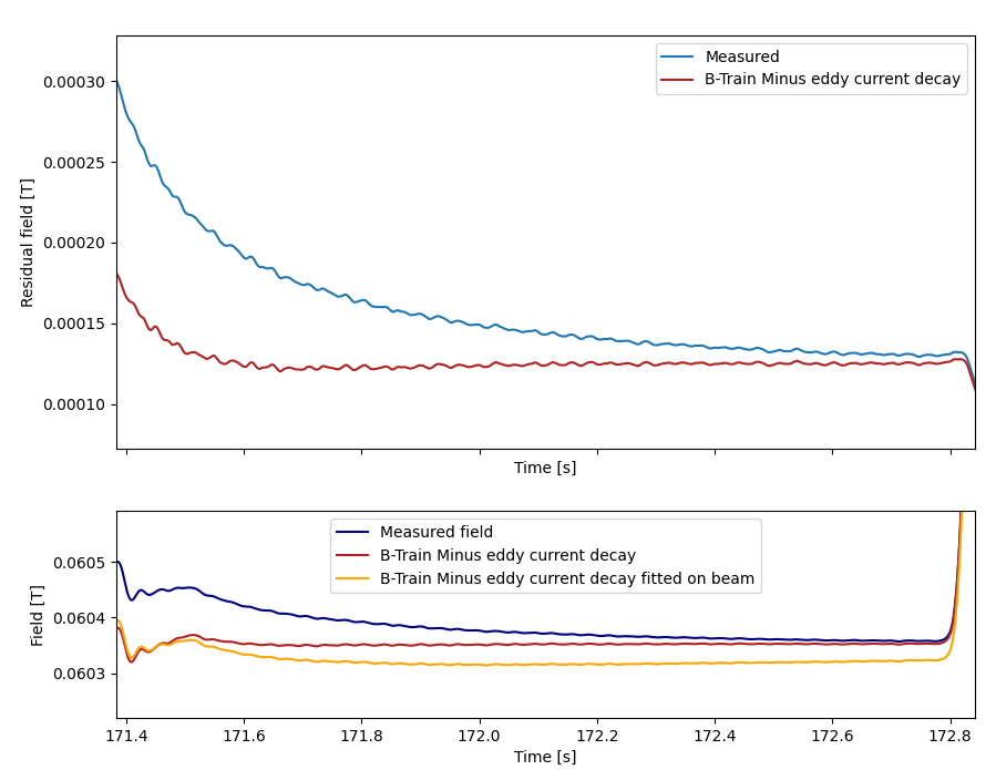
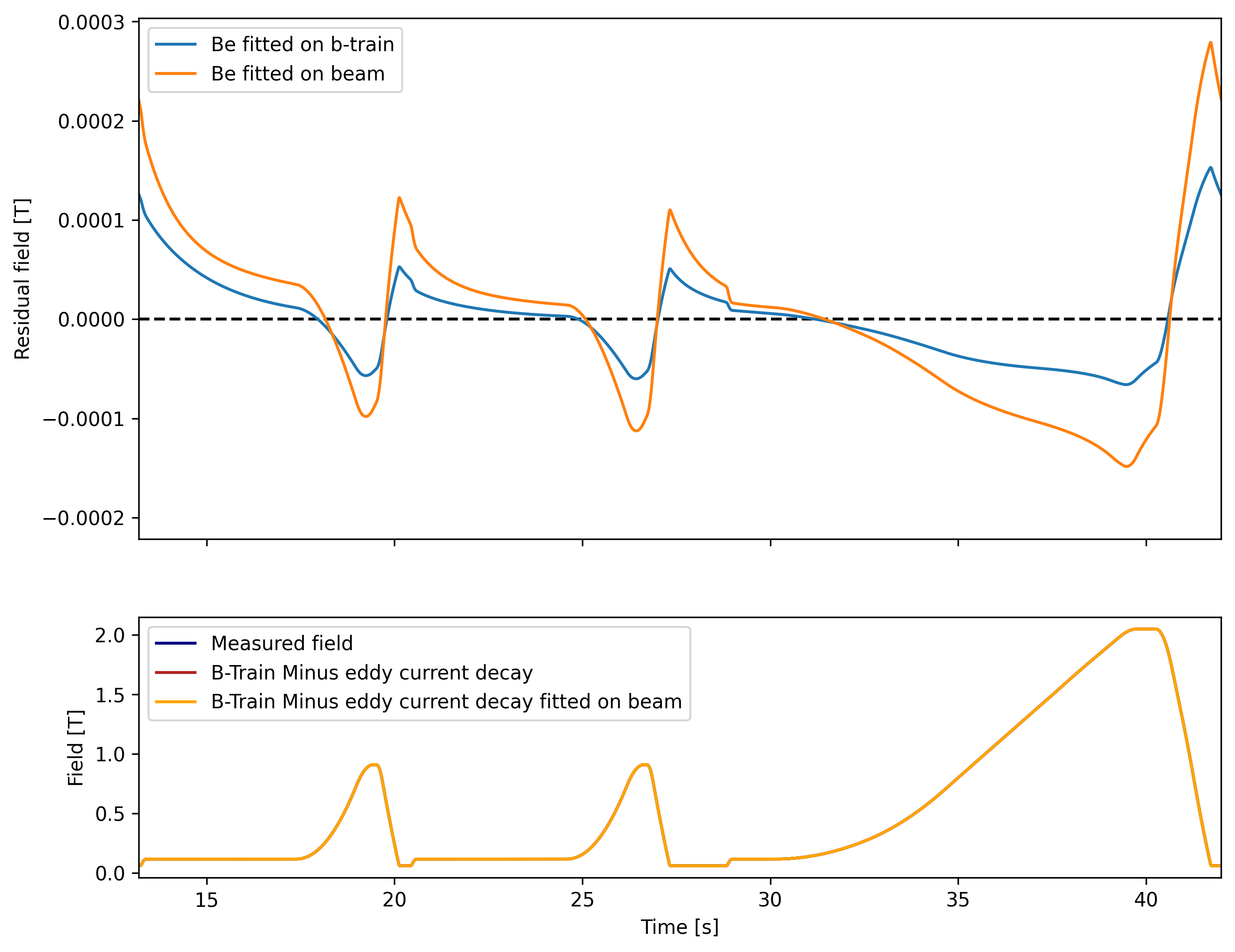
Based on the eddy current fit we see that the decay is subtracted sufficiently well up to linear drift. We use this approach to make Dipole dataset v7.

Decay on orbit measurements

We retrieve the data from the MD2 orbit decay from 2025-03-27 and fit only ${\tau }_2,{\tau }_3$ on the MD2 orbit since we assume ${\tau }_1$ is fast decaying. Additionally we retrieve SFTION1 (O4) data from Eddy current measurements 2025-06-27 when the injection plateau was still constant (and also constant RF at injection). We also retrieve data from LHCION3 from 2025-07-02 to use as validation.

In all, we fit time constants on the following datasets

• SFTPRO1 (after MD5)
• SFTPRO1 (after LHCINDIV)
• MD2 (6 BP MD cycle)
• SFTION1 (after MD1)
• LHCION3

We validation on another SFTION1 dataset but this one measured after an LHCINDIV.

N.B. LHCION3 BPMs seem to be recording at 3ms interval (333 Hz)

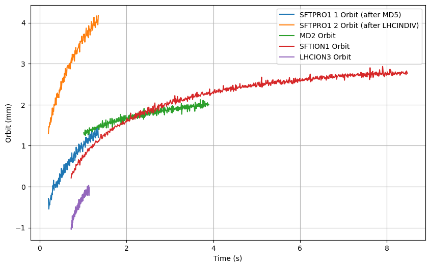Fitting with 2 or 3 exponentials using differential evolution we receive

2 exponential fit results

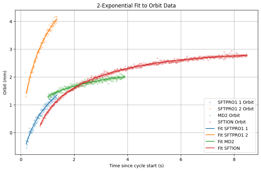Objective score: 3.424 Number of iterations: 6646

Parameter	Value (seconds)	Description
tau1	0.569829	Fast time constant (only in orbits 1 & 2)
tau2	2.79074	Medium time constant (all orbits)

Time Constant	Orbit 1 Coefficient	Orbit 1 Contribution (%)	Orbit 2 Coefficient	Orbit 2 Contribution (%)	MD2 Orbit Coefficient	MD2 Orbit Contribution (%)	SFTION Orbit Coefficient	SFTION Orbit Contribution (%)
tau1	-1.15049	34.4142	-1.88816	37.9804	-0.124693	12.054	-0.705517	26.9034
tau2	-2.19258	65.5858	-3.08325	62.0196	-0.909761	87.946	-1.91689	73.0966

In this optimization we remove the restriction to force ${\tau }_1<0.5$ and let the optimization choose freely.

3 exponential fit results

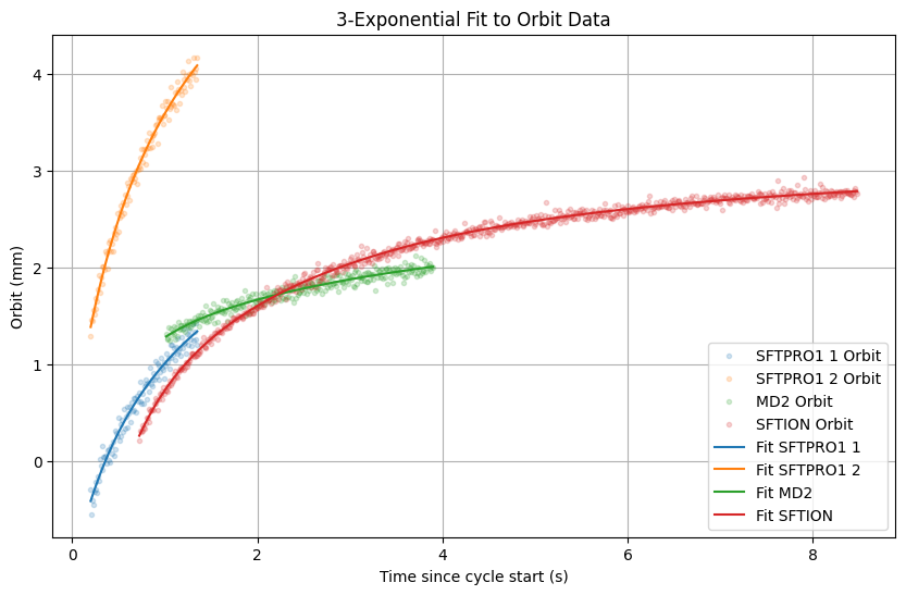Objective score: 3.413 Number of iterations: 40000

Parameter	Value (seconds)	Description
tau1	0.369691	Fast time constant (only in orbits 1 & 2)
tau2	1.7	Medium time constant (all orbits)
tau3	7.92859	Slow time constant (all orbits)

Time Constant	Orbit 1 Coefficient	Orbit 1 Contribution (%)	Orbit 2 Coefficient	Orbit 2 Contribution (%)	MD2 Orbit Coefficient	MD2 Orbit Contribution (%)	SFTION Orbit Coefficient	SFTION Orbit Contribution (%)
tau1	-0.548754	16.9138	-0.904994	19.4348	0	0	-0.888689	31.2587
tau2	-2.42163	74.6399	-3.7297	80.0954	-0.0875694	16.4726	-0.384908	13.5387
tau3	-0.274036	8.44637	-0.0218763	0.469793	-0.444036	83.5274	-1.56942	55.2026

We see only an improvement of about 1 % in objective score using 3 exponentials over 2 exponentials.

Validation

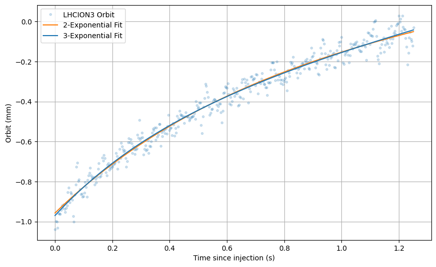
	Objective score	Validation score
2-Exponential	3.42375	0.806774
3-Exponential	3.41327	0.798459

We find the 2-exponential to not fit so well.

Fitting first turn data

We use various notebooks to retrieve the radial offset, theoretical db offset and IREF and save to intermediate dataframes and load into a curve fitting notebook

Notebooks

• MD20250627/bpm-data-sftion-1.ipynb
• MD20250627/bpm-data-sftion-2.ipynb
• MD20250709/bpm-data-md5.ipynb
• MD20250709/bpm-data-sftpro1-1.ipynb
• MD20250709/bpm-data-sftpro1-2.ipynb

Fitting notebook

• MD20250709/exponential-convolution-fitting.ipynb

Plotting the first turn radial offsets, we see the following:

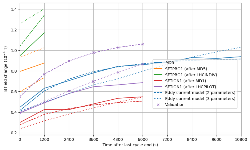We fit parameters using differential evolution and sampling parameters in log-space, and forcing the coefficients to be negative (since the eddy current contributions should be decaying negatively)

	Objective score	C1	C2	C3	TAU1	TAU2	TAU3
Double fixed	0.326535	-0.000918377	-0.000350356	nan	0.532	2.72	nan
Triple fixed	0.288963	-0.00147969	-0.000161257	-0.000352203	0.415	1.745	9.433
BFGS fit 2	0.106625	-0.000914974	-0.000350089	nan	0.532	2.72	nan
BFGS fit 3	0.0834998	-0.00147243	-0.00016114	-0.000352065	0.415	1.745	9.433

Notes

• Cannot use pure scipy.minimize with jacobian for exponential coefficients, since this does not enforce coefficients to be negative
• multi objective optimization with evolutionary algorithms does not work for fitting every parameter because we have 20+ parameters, and this is too high dimensional to converge properly
• Pure gradient descent gets stuck in local minima.
• Best to use evolutionary algorithms and moo for time constants, and use varpro or similar algorithms to fit the coefficients analytically with least squares, since the coefficients and offsets present a linear problem, and the time constants are nonlinear.