Multi-objective optimization for eddy current parameter fitting
Since the Eddy current decay problem in the SPS Main Dipoles pose a complex optimization problem, having to fit exponentials with shared time constants between exponential convolutions / sums (cumulative eddy current contributions) on first turn data, and orbit decays, we are effectively balancing two losses and as .
With differentiable optimization, we can assign weights as static values (e.g. 1 and 1, or put higher weights on orbit, e.g. 1 and 5), however biases the solution towards prior knowledge, and may yield solutions which are suboptimal if the optimization does not converge to a global optimum, or if a global optimum does not exist. In our case, a global optimum might not exist if the phenomelogical model does not fit the data.
As with previous experiments we fit the data to 1, 2 and 3 exponentials to determine which system fits the data best, since no prior knowledge about the system exists.
Datasets
We load the datasets we have consisting of
Convolution data
- SFTPRO1_1
- SFTPRO1_2
- SFTPRO1_3
- SFTPRO1_4
- SFTION1_1
- SFTION1_2
- MD5
Each dataset is a list of dictionaries each with
- for a corresponding
- and
Since we are looking at the first turn decay
Orbit data
- SFTPRO1 (after XXX)
- SFTPRO1 (after YYY)
- MD2
- SFTION1
- LHCION3
Each dataset is a set of for an orbit decay over a full injection plateau, normally > 100 points. The length of the arrays depend on the resolution of the BPMs at that time, and the length of the injection plateau.
Data preprocessing
And convert the to using
Which uses the chain rule for
Where is simply a calibration function.
Hyperparameters
We use a Genetic Algorithm from pymoo NSGA-II with the following hyperparameters
1 exp
pop_size: 400
n_gen: 500
seed: 42
2 exp
pop_size: 400
n_gen: 2000
seed: 42
3 exp
pop_size: 400
n_gen: 4000
seed: 42
Parameter bounds
The NSGA-II algorithm supports bounds bounds, and we need to keep the optimized parmeters physical.
For the time constants we apply seconds. For the orbit decay coefficients we apply For the orbit offsets we apply For the convolution coefficients we apply .
Parameter initializations
We use smart parameter initializations, using found from Eddy current decay in the SPS main dipoles, and orbit offsets from the data.
# 1-exponential model initial parameters
INITIAL_PARAMS_1EXP = {
    "tau": [0.8],
    "orbit_coefficients": [[-3.0], [-4.7], [-0.7], [-2.4], [-1.2]],
    "orbit_offsets": [2.5, 6.0, 2.0, 2.5, 0.4],
    "conv_coefficients": [-3.0],
    "qf_conv_coefficients": [-1e-4],  # Only used if OPTIMIZE_QF=True
}

# 2-exponential model initial parameters (when no previous result)
INITIAL_PARAMS_2EXP = {
    "tau": [0.53, 2.72],
    "orbit_coefficients": [
        [-1.4, -0.6],
        [-1.75, -0.75],
        [-2.1, -0.9],
        [-1.96, -0.84],
        [-0.35, -0.15],
    ],
    "orbit_offsets": [3.0, 7.0, 2.5, 3.0, 0.5],
    "conv_coefficients": [-0.07, -0.03],
    "qf_conv_coefficients": [-0.035, -0.015],  # Only used if OPTIMIZE_QF=True
}

# 3-exponential model initial parameters (when no previous result)
INITIAL_PARAMS_3EXP = {
    "tau": [0.43, 1.81, 6.76],
    "orbit_coefficients": [
        [-1.26, -0.42, -0.28],
        [-1.575, -0.525, -0.35],
        [-1.89, -0.63, -0.42],
        [-1.764, -0.588, -0.392],
        [-0.315, -0.105, -0.07],
    ],
    "orbit_offsets": [3.0, 7.0, 2.5, 3.0, 0.5],
    "conv_coefficients": [-0.07, -0.03, -0.021],
    "qf_conv_coefficients": [-0.0245, -0.009, -0.0049],  # Only used if OPTIMIZE_QF=True
}

# =============================================================================
# INITIALIZATION FROM PREVIOUS RESULTS
# =============================================================================

# Scaling factors for initializing from previous results
PREV_RESULT_SCALING = {
    "2exp_from_1exp": {
        "tau_values": [0.53, 2.72],  # Optimized tau values
        "orbit_coeff_split": [0.7, 0.3],  # Split 1-exp coeffs
        "conv_coeff_split": [0.7, 0.3],
        "qf_conv_coeff_split": [0.7, 0.3],  # Only used if OPTIMIZE_QF=True
    },
    "3exp_from_2exp": {
        "tau_values": [0.43, 1.81, 6.76],  # Optimized tau values
        "orbit_coeff_split": [0.9, 0.7, 0.2],  # Split 2-exp coeffs
        "conv_coeff_split": [0.7, 0.7, 0.3],
        "qf_conv_coeff_split": [0.7, 0.3, 0.2],  # Only used if OPTIMIZE_QF=True
    },
}
Results
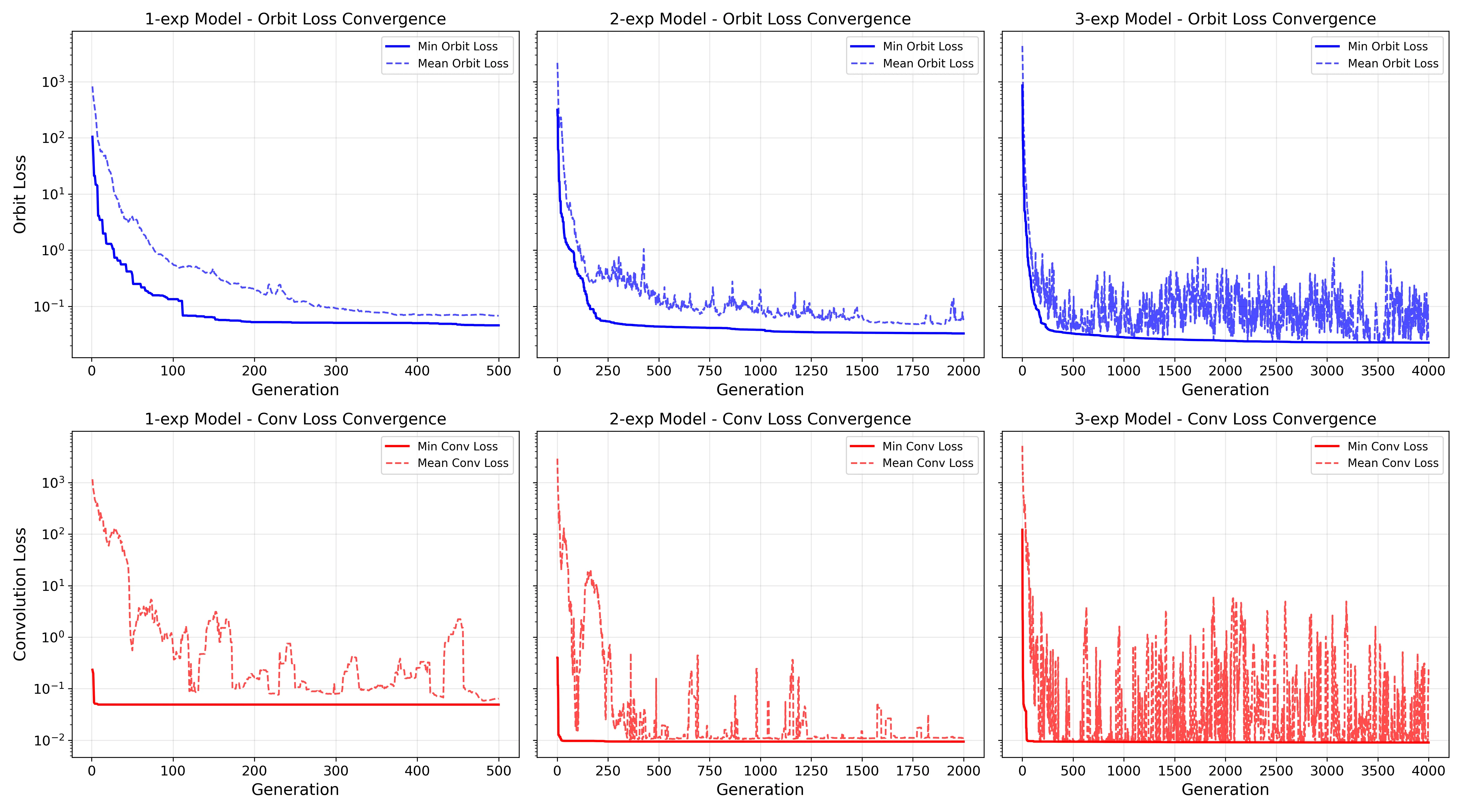
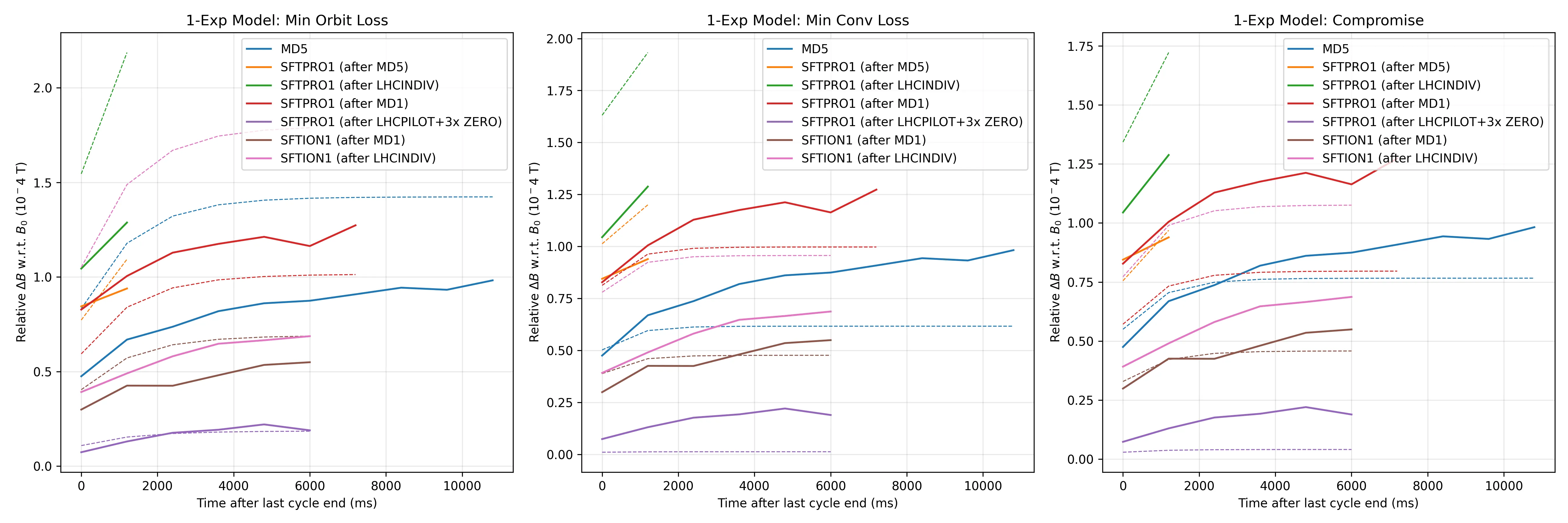
Without taking into account the QF contribution, the objectives converge as follows:
| Model | Population Size | Generations | Pareto Solutions | Pareto Ratio | Min Orbit Loss | Max Orbit Loss | Min Conv Loss | Max Conv Loss |
|---|---|---|---|---|---|---|---|---|
| 1-exp | 400 | 500 | 107 | 26.8% | 0.0459 | 0.0942 | 0.049 | 0.2518 |
| 2-exp | 400 | 2000 | 238 | 59.5% | 0.0329 | 1.6666 | 0.0094 | 0.0491 |
| 3-exp | 400 | 4000 | 42 | 10.5% | 0.0226 | 0.0541 | 0.009 | 0.0495 |
Plotting the pareto fronts from the optimization shows the following, with logarithmic scale.
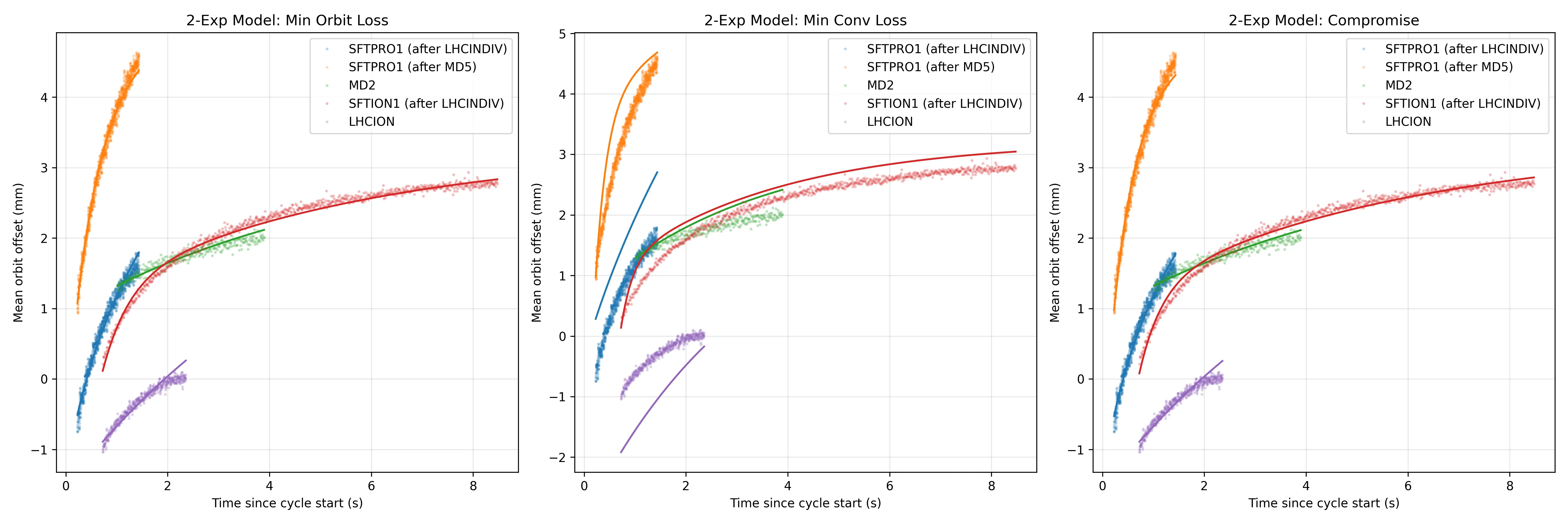
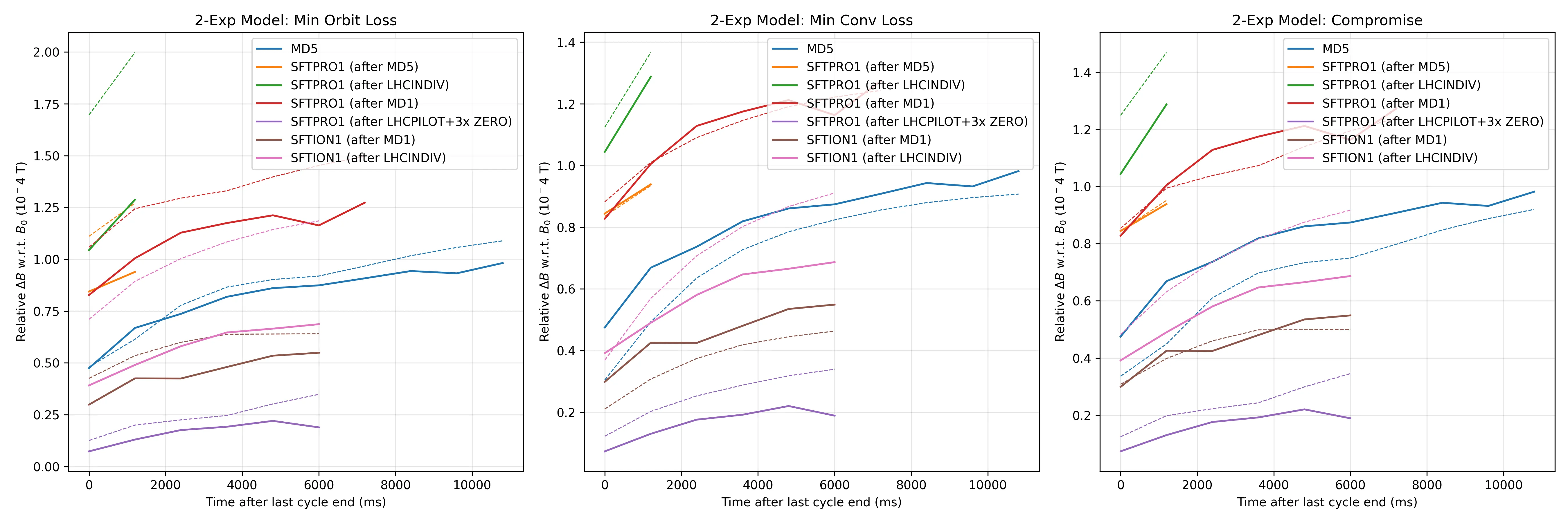
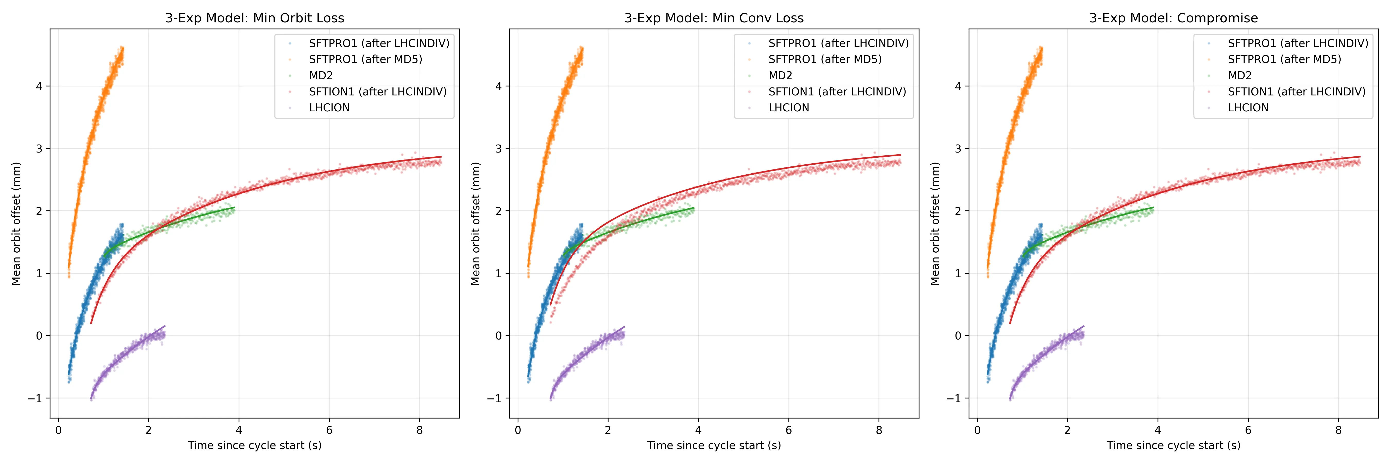
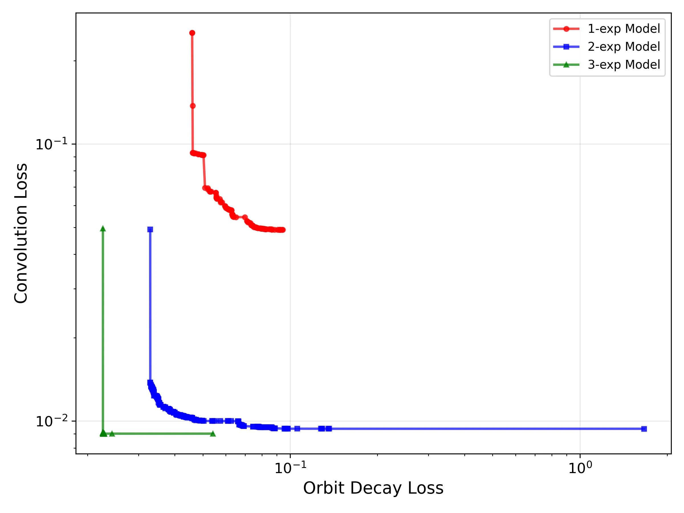 It’s clear that as we add more exponentials, the loss decreases. However zooming into the bottom left corner of the 3-exp optimization we see
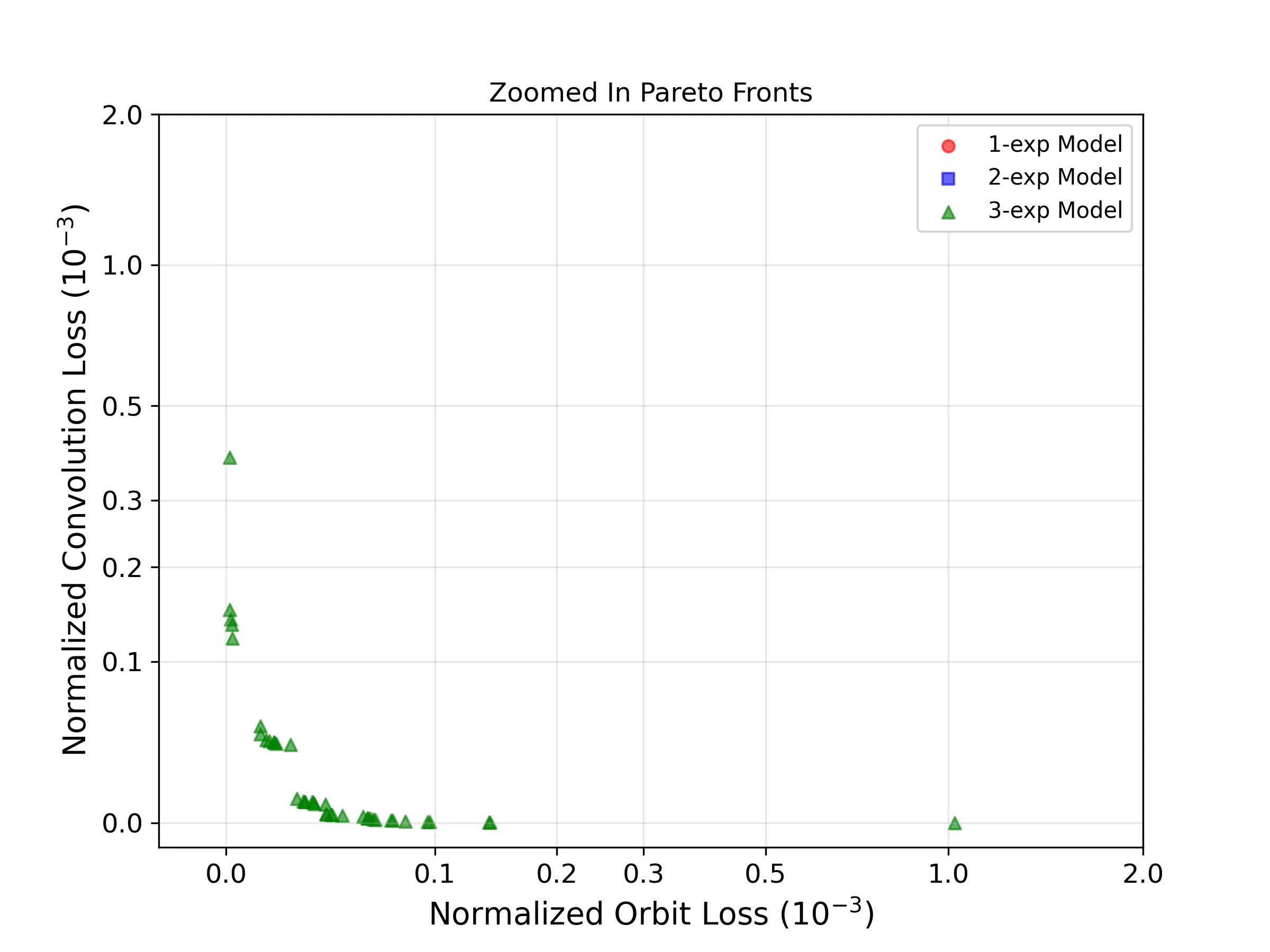
Clearly in this optimization there is no global optimum, and we are forced to choose a compromise solution.
We use an interactive selector to select the solution in the corner.
| Model | Orbit Loss | Conv Loss | Total Loss | Normalized Distance | Tau Values | Main Conv Coeffs |
|---|---|---|---|---|---|---|
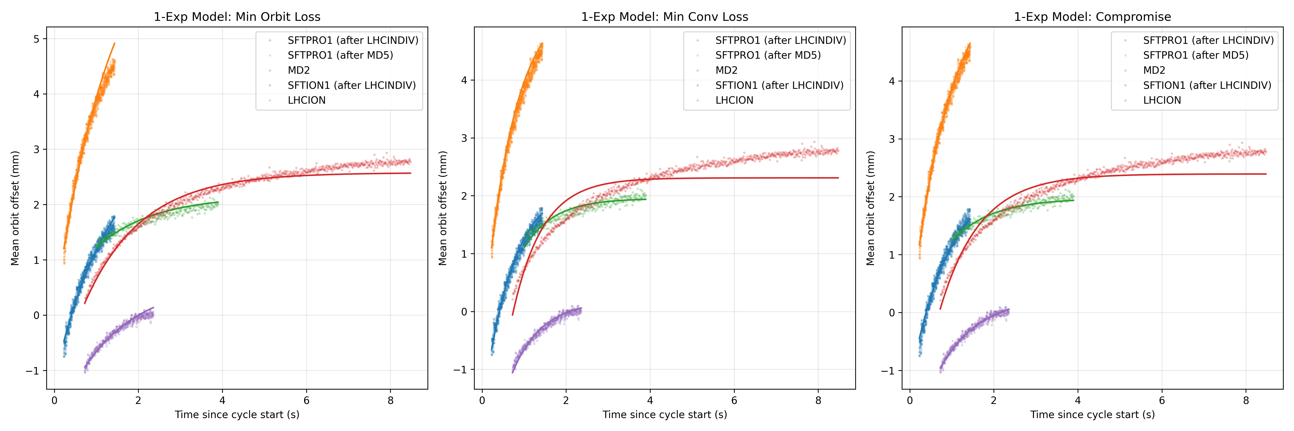
| 1-exp | 0.0864818 | 0.049047 | 0.135529 | 0.169451 | 1.015 | -2.723 |
| 2-exp | 0.0371244 | 0.0111024 | 0.0482269 | 0.0123567 | 0.373, 4.599 | -6.345, -0.952 |
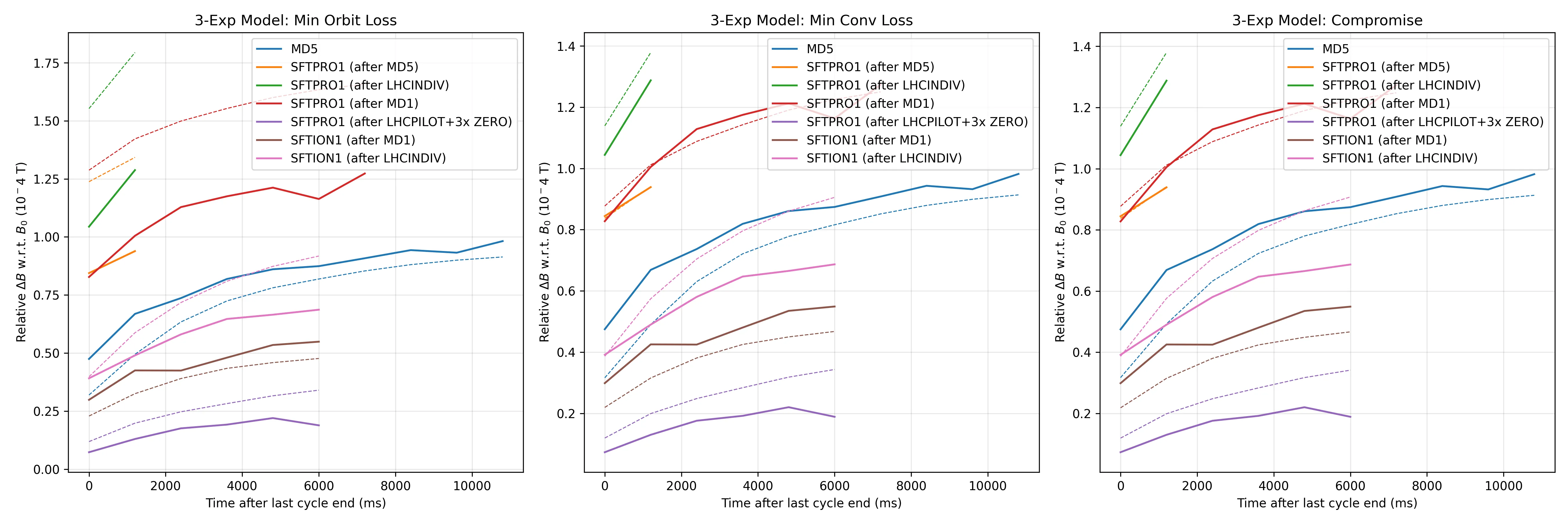
| 3-exp | 0.0226398 | 0.0090084 | 0.0316482 | 2.87467e-05 | 3.535, 0.419, 0.113 | -0.962, -2.303, -156.282 |
1 exponential fit
2 exponential fit
3 exponential fit
3 exponential fit errors
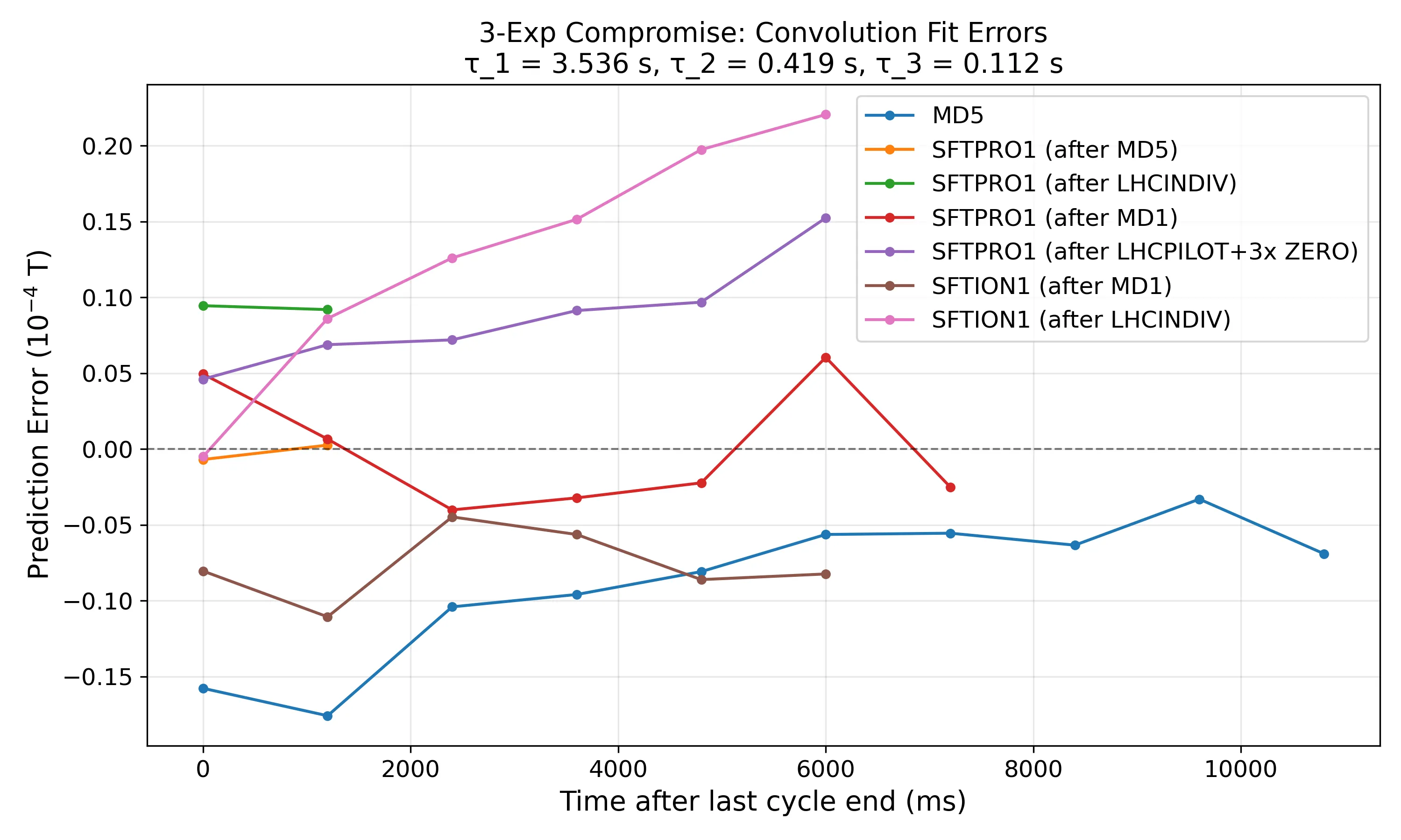
The maximum error on the conv loss is ca Tesla on an SFTION cycle, which translates to roughly 0.6 mm first turn difference.