We can fit a differentiable Preisach model to SPS Main Dipole measured data from the B-Train to create datasets that can be used for pre-training neural networks.
Results
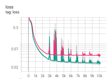
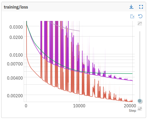
purple mesh_scale=0.1 green mesh_scale=0.5 gray mesh_scale=0.1
Mesh scale 0.1 - 7411 points
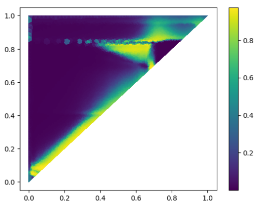
Single quadrant
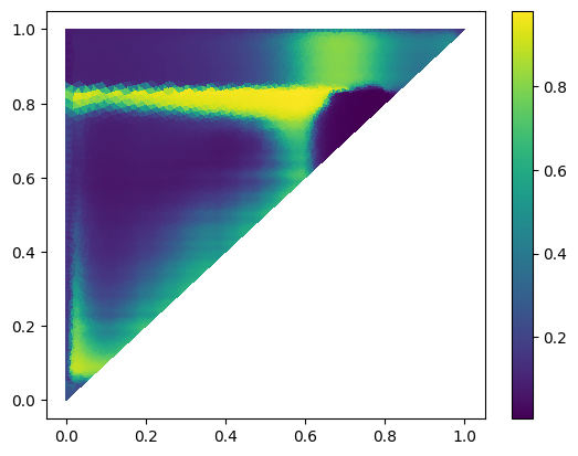
We restrict the domain to instead of . This results in the the diagrams below, where only 1/4 of the triangle gets painted.
Mesh scale: 0.5
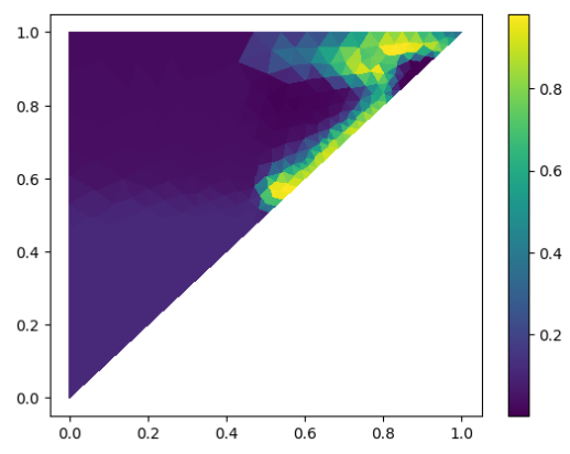
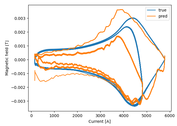
Mesh scale: 0.1
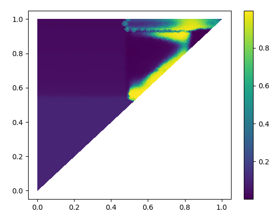
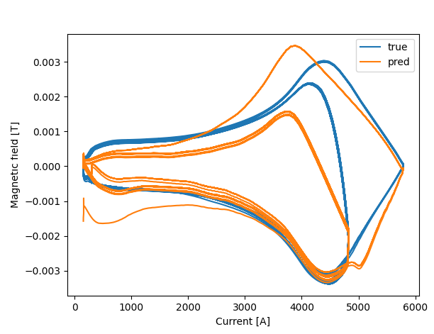
Changing calibration function
By changing calibration function from v4 to v6 we improve the loss by an additional 10%
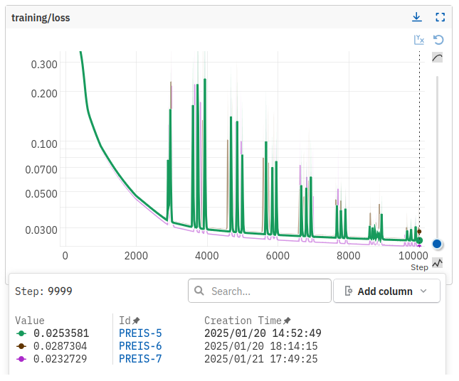
Dynamic effects
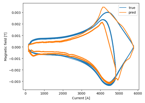
The used Preisach model does not at all consider dynamic effects, whereas this is present in training data due to Eddy current decay. I.e. the field is changing while the current stays constant.
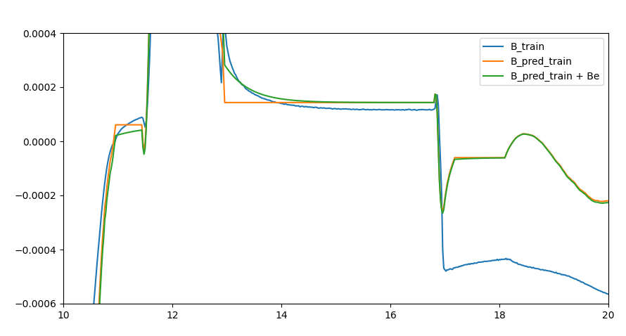
As seen in the figure, significant eddy currents can be seen after ramp down (in the middle in the figure), as well as decay at flat top (to the left), but also some drift is visible (to the right). We could fit data from 867 measurements that show less dynamic effects, however the data is signficantly noisier.
Here we add eddy currents with the following parameters:
eddy_params = {
    "alpha": .4e-4, # tau_e = alpha * H + beta, inverse reduction of Ie -> larger -> faster decay
    "beta": 0.45,  # larger -> faster decay
    "tau_em": 1.9e-4,  # contribution from H -> larger -> more "new" eddy currents
    "c": 0.0004,
}
Fitting to MBA data
We fit the Peisach model to MBA data measured from Average multiple measurements for noise reduction since it contains less dynamic effects, and fit a hysteron density like
And a fitted phase-space like
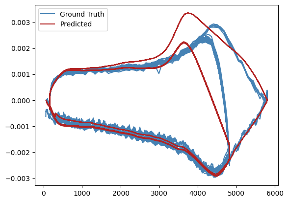
With a downsampling rate of 20 (1 kHz → 50 Hz). Even considering the noise of the data, the model fits rather noise-free hysteresis loops after just 2000 iterations / epochs. Further training of the model overfits with the following plots:
In terms of model accuracy we see the following
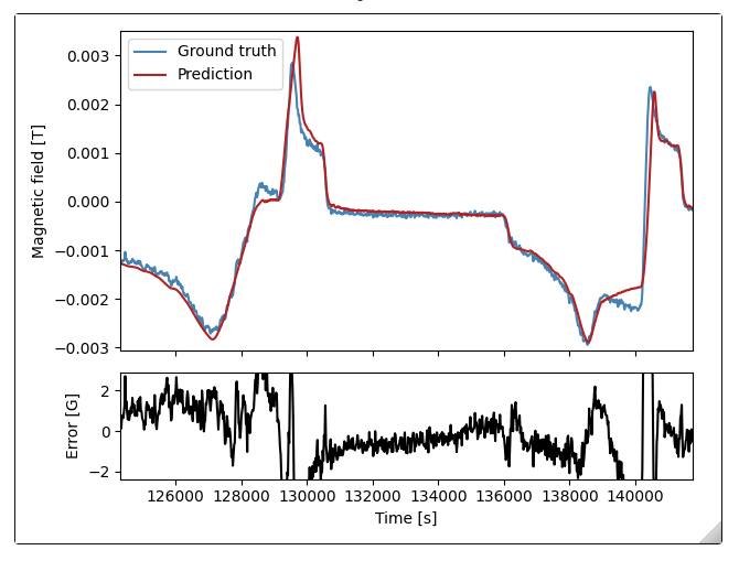
We see that the accuracy stays around 2G overall.
Computing the MAE and RMSE
| RMSE (e-4 T) | MSE (e-4 T) | |
|---|---|---|
| Global | 2.63 | 1.20 |
| Beam in | 1.60 | 1.07 |
We see a big improvement in RMSE, but still well above 1 G, which is not yet sufficient for hysteresis compensation at flat bottom.
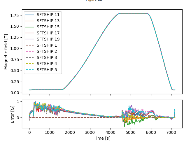
Plotting the predicted fields overlayed (to show some form of hysteresis), with the first field chosen as reference, and cycles 11-19 are nestled between LHCPILOTs (LHC type supercycle), we see that the model is unable to predict the 2 G hysteresis that is supposed to be present during supercycle changes, which might suggest that the model is unable to perfectly fit this behaviour, although input noise in the measured current can certainly account for this effect as well.
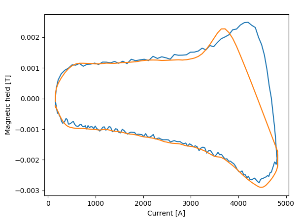
As seen in the figure, the model follows the ramp well, but the source data is not clean enough for a good fit.
10000 iterations
Fitting the same model 10000 iterations we recover
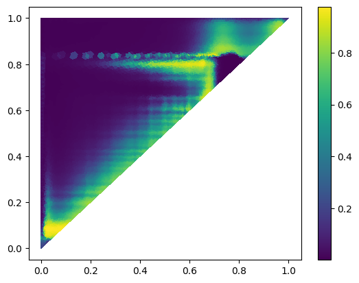
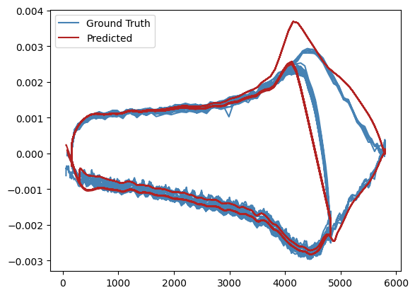
We see that unphysical artifacts are introduced at 5000 A, ramping up the LHCPILOT cycle, as well as rippling effects during ramps. For this reason we use the model fitted to 2000 epochs.
Adding a linear component to the hysteresis
We observe that there are significant artifacts in the inferred field,
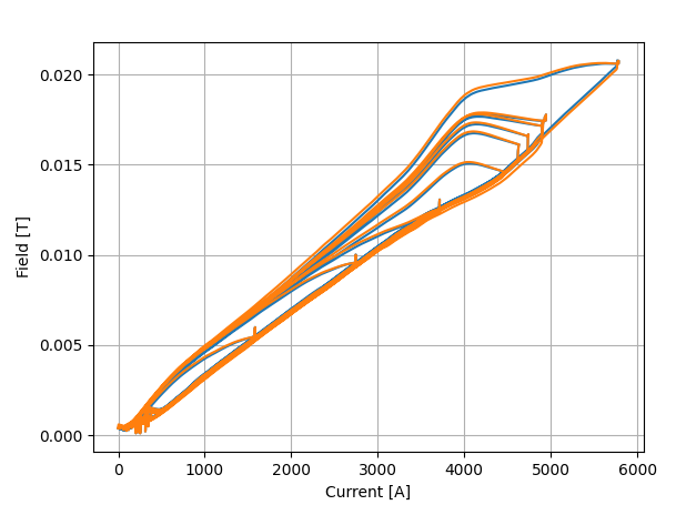
After adding the linear component we still see artifacts on the turning points, unfortunately.