Adaptive downsampling on simulated data

In preparation for training with irregular time indices, with simulated data data will be adaptively downsampled with RDP.

Running RDP on the datasets

"~/cernbox/hysteresis/dipole/datasets/simulation/train_piecewise_eddy_24h.parquet"
"~/cernbox/hysteresis/dipole/datasets/simulation/train_piecewise_eddy_1h.parquet"
"~/cernbox/hysteresis/calibration_fn/SPS_MB_I2B_CALIBRATION_FN_EDDY_SIM.csv"
 

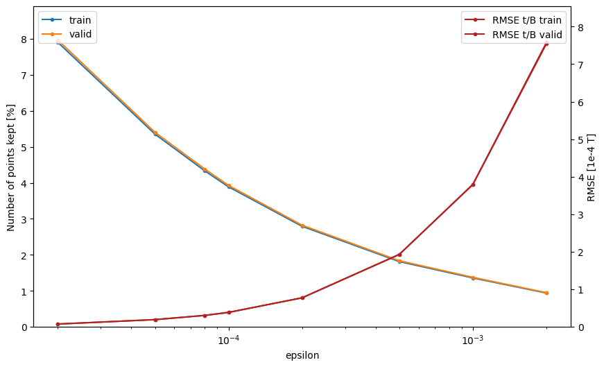
after subtracting a piecewise linear function and normalizing, with different values of $\epsilon \in [2e-5,5e-5,8e-5,1e-4,5e-4,1e-3,2e-3]$ .

The masks are saved in the training and validation dataframes in

~/cernbox/hysteresis/dipole/notebooks/dynamic-downsampling/processed_dataframes/train_sim_df.parquet ~/cernbox/hysteresis/dipole/notebooks/dynamic-downsampling/processed_dataframes/val_sim_df.parquet

Using $\epsilon$ between $2\times 10^{-5}$ and $2\times 10^{-3}$ makes effective downsampling between 10 and 100, however with $\epsilon >5\times 10^{-4}$ makes the RMSE increase drastically. Therefore the max $\epsilon$ that should be used is $5\times 10^{-4}$.

Preventing large time gaps

When large amounts of continuous points are removed, the time gap can be large, making $\Delta t$ outliers, that worsens the granularity of $\Delta t$ when normalized. Therefore there is need to re-add back points that are outside of $2\sigma$.

Points are added evenly distributed with a random gap size where there are large time skips. This adds between $0.05\%$ and $0.5\%$ points, but reducing the maximum time value from 3000+ to below 500, which gives a time dynamic range of 0-500.

The following is from a jupyter notebook where timesteps are added:

Average time step size

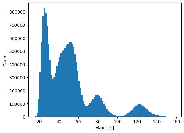
For the optimal $\epsilon =5\times 10^{-4}$, the average median step is 36 ms. With a sequence length of 600 this equates to 21s of data on average.

With a context sequence length of 1200 and target sequence length of 600 we get

distribution