Problem
In Fit piecewise-linear fn to I-B v1 and Fit piecewise-linear fn to I-B v2 the calibration function is further tuned to experimental data, however the fit especially at flat top remains poor.
Outcome
This development further improves the fit of the discrete function by making it possible to drag and drop calibration function points in an interactive matplotlib graph. Additionally and automatic fit is done my taking the average between the field in the magnetization and demagnetization directions at points where the calibration function is defined.
The code for visualizing and fitting the calibration function is somewhat generic and bundled in the Calibration Function Tuner Python package (GitLab install only)
Results
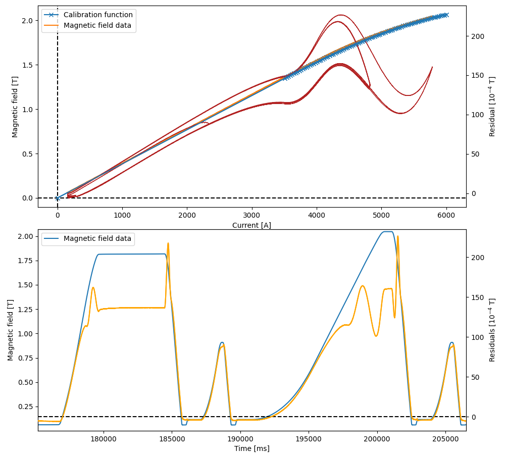
Default LSA calibration function
tune-calibration-fn -c ~/cernbox/hysteresis/calibration_fn/SPS_MB_B2I_CALIBRATION_FN_LSA.csv
The residual ranges from 0 to 200 G, with many ripples that are not entirely physical due to the miscalibration of the function.
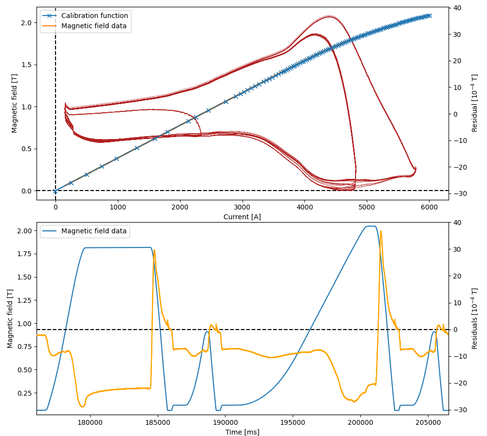
Improved calibration function (v2)
tune-calibration-fn -c ~/cernbox/hysteresis/calibration_fn/SPS_MB_I2B_CALIBRATION_FN_v2.csv
Here we clearly see an improvement with +/- 35G (70 G range), still with some large deviations from 0 in both positive and negative direction. Especially at LHCPILOT flat top the offset is too much in the negative in magnitude. This indicates a potential shift in the calibration function.
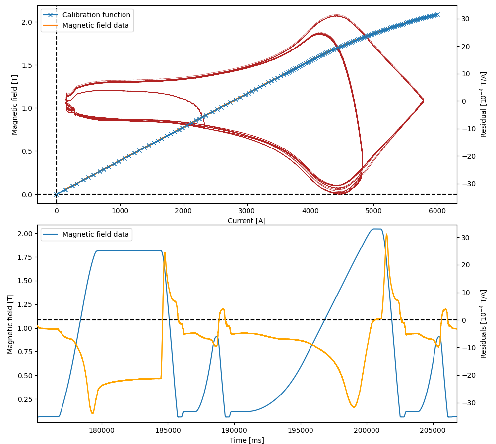
Improved calibration function (v3)
Proposed in this experiment by first making an automatic fit, and then tuning the points manually in the interactive plot.

It is shown that the major effects are during ramps, which correspond to the lagging effects caused by eddy currents, whereas flat bottom are not as pronounced.
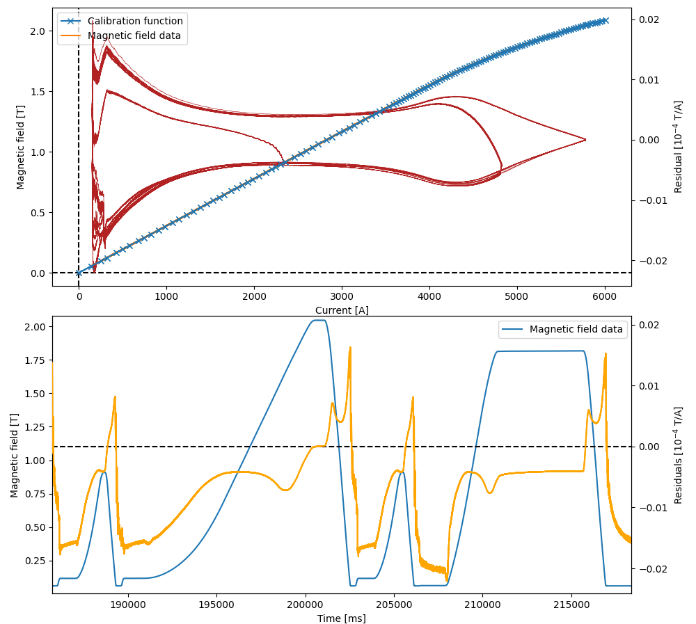
As remedy for the drowning out caused b eddy currents we plot also B/I vs I as seen below, where flat bottom has significantly larger effects than the rest of the cycle.
