Since SFTPRO1 injects at 200 ms, we see the fastest decaying effects on this beam only (as opposed to on LHC-type cycles at 1015 ms, and ion cycles at 725 ms)
Using orbits from BC MD 2025-03-18:
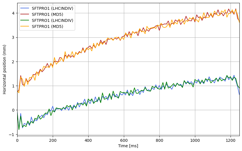 We fit 1-3 exponentials on the orbits following LHCINDIV:
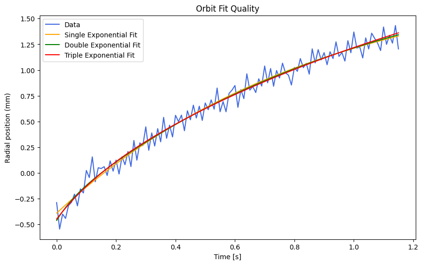
And after MD5:
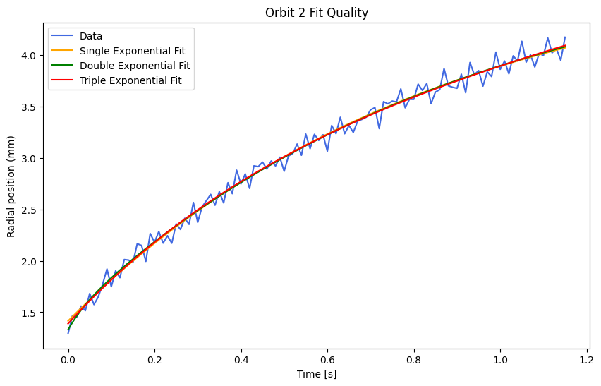
Using differential evolution and bounding the decay constants to be positive, and all exponential coefficients to be negative
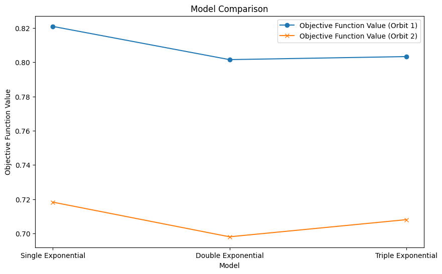
We see in both cases that the fit quality is best with 2 exponential contributions.
| Model | Orbit 1 Parameters | Orbit 1 Score | Orbit 2 Parameters | Orbit 2 Score |
|---|---|---|---|---|
| Single Exponential | -2.359968, 0.879717, 1.968803 | 0.820975 | -3.560503, 0.840908, 4.975826 | 0.718298 |
| Double Exponential | -0.138364, 0.060004, -2.497912, 1.045346, 2.174302 | 0.801566 | -0.136647, 0.040736, -3.647105, 0.913171, 5.114687 | 0.698041 |
| Triple Exponential | -0.125303, 0.058215, -7.581678, 21.302642, -1.671180, 0.786894, 8.917537 | 0.803347 | -1.716310, 0.485100, -1.389217, 5.004211, -8.505133, 10.766929, 12.999666 | 0.708055 |
| SFTPRO ramps until 102 ms, and injects at 200 ms, so any effects with time constant s or longer should be visible at injection. |
In principle we should see the same eddy current decay constants for both cycles, but we do not, so we proceed with fitting shared decay constants, and independent exponential coefficients
Fitting shared
We use differential evolution from scipy to fit this non-convex problem using code like
# Define the multi-exponential model with shared time constants
def multi_exponential_shared(t, tau1, tau2, C1_orbit1, C2_orbit1, C1_orbit2, C2_orbit2, C_offset1, C_offset2) -> tuple[npt.NDArray[np.float64], npt.NDArray[np.float64]]:
    exp1_orbit1 = C1_orbit1 * np.exp(-t / tau1)
    exp2_orbit1 = C2_orbit1 * np.exp(-t / tau2)
    exp1_orbit2 = C1_orbit2 * np.exp(-t / tau1)
    exp2_orbit2 = C2_orbit2 * np.exp(-t / tau2)
    return exp1_orbit1 + exp2_orbit1 + C_offset1, exp1_orbit2 + exp2_orbit2 + C_offset2

# Define the objective function for optimization
def objective_function(
    params: npt.NDArray[np.float64],
    t: npt.NDArray[np.float64],
    orbit1_fit: npt.NDArray[np.float64],
    orbit2_fit: npt.NDArray[np.float64]
) -> float:
    tau1, tau2, C1_orbit1, C2_orbit1, C1_orbit2, C2_orbit2, C_offset1, C_offset2 = params
    fit_orbit1, fit_orbit2 = multi_exponential_shared(t, tau1, tau2, C1_orbit1, C2_orbit1, C1_orbit2, C2_orbit2, C_offset1, C_offset2)
    error_orbit1 = np.sum((orbit1_fit - fit_orbit1)**2)
    error_orbit2 = np.sum((orbit2_fit - fit_orbit2)**2)
    return error_orbit1 + error_orbit2

# Initial guesses and bounds
bounds = [
    (TAU_MIN, TAU_MAX),  # tau1
    (TAU_MIN, TAU_MAX),  # tau2
    (C_MIN, C_MAX),      # C1_orbit1
    (C_MIN, C_MAX),      # C2_orbit1
    (C_MIN, C_MAX),      # C1_orbit2
    (C_MIN, C_MAX),      # C2_orbit2
    (-OFFSET_RANGE, OFFSET_RANGE),  # C_offset1
    (-OFFSET_RANGE, OFFSET_RANGE)   # C_offset2
]

result_multi2 = scipy.optimize.differential_evolution(
    objective_function,
    bounds=bounds,
    args=(t_fit, orbit1_fit, orbit2_fit),
    maxiter=10000,
    popsize=25,
    tol=1e-6,
    mutation=(0.5, 1.5),
    recombination=0.7,
    seed=42,
    disp=True
)
Where we ensure that the we set bounds so that the time constants and coefficients are physical.
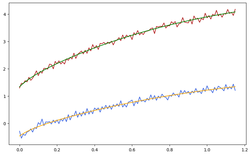
With 3exponentials we fit the following:
| Parameter | Orbit 1 Value | Orbit 2 Value |
|---|---|---|
| tau1 | 2.286 s | 2.286 s |
| tau2 | 2.019 s | 2.019 s |
| tau3 | 0.060 s | 0.060 s |
| C1 | 32.458 | 61.052 |
| C2 | -33.362 | -61.495 |
| C3 | -0.148 | -0.169 |
| C_offset | 0.588 mm | 1.951 mm |
With 2 taus
| Parameter | Orbit 1 Value | Orbit 2 Value |
|---|---|---|
| tau1 | 0.053 s | 0.053 s |
| tau2 | 0.956 s | 0.956 s |
| C1 | -0.108 | -0.157 |
| C2 | -2.406 | -3.708 |
| C_offset | 2.057 mm | 5.200 mm |
| In principle we see for the 3exp fit that tau1 and tau2 are very similar, and that the C1 and C2 coefficients partially negate each other, and the results don’t agree fully with when we fit only 2 exponentials. We realize we need additional data to fit the time constants across more orbit decays. |