Eddy current decay in the SPS main quadrupoles

Decay on the reference magnet

Based on measurements performed 2025-07-14 in the SPS quadrupole bench in 867, where we divide the waveforms into static plateaus, essentially keeping the idle current, (LHC) injection plateau, and flat tops. In this case we get a long plateau after each ramp, and we see strong eddy current decays

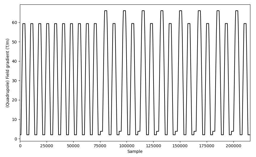Zooming in to the first ramp-down

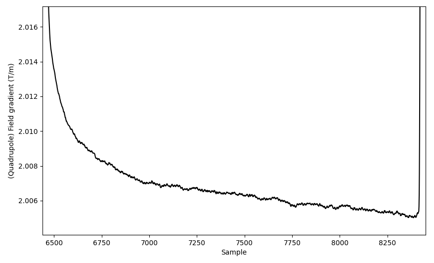
Similarly we see a decay at the start of flat top. Each sample is spaced 1 ms apart (1 kHz sampling freqency), so we have about 1.7s of data for each decay. We see the following for both the ramp-up and ramp-down:

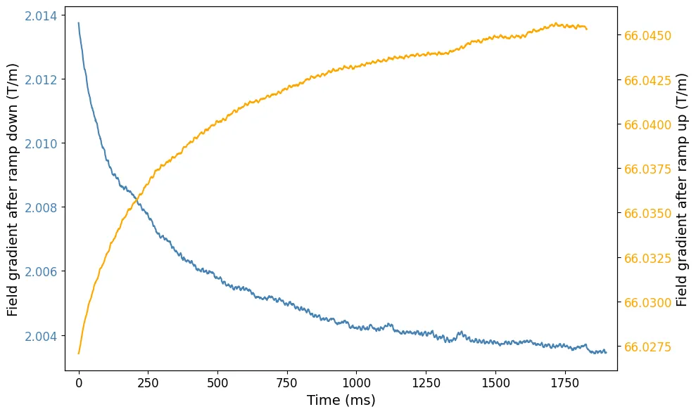
We apply scipy.optimize.curve_fit to fit exponentials to the decays, and use single and double exponential to see what fits better. We also add a linear term for the fit to account for approximately linear integration drift. The coefficients are constrained to be positive for the decay down, and positive for the decay up, and the constant can be any sign.

model	decay	${\tau }_1$ (ms)	${\tau }_2$ (ms)	RMSE
1-exp	down	$232$		$1.55\times 10^{-4}$
1-exp	up	$249$		$1.55\times 10^{-4}$
2-exp	down	$41$	$342$	$8.42\times 10^{-5}$
2-exp	up	$50$	$306$	$1.11\times 10^{-4}$

Then we apply joint optimization to optimize the time constants jointly for the two decays, since they describe the same physical system, which yields the following fits:

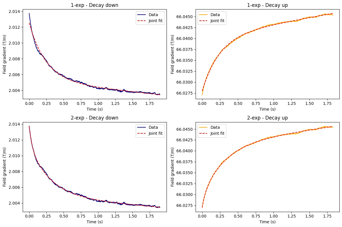
The following table summarizes the optimization

model	decay	${\tau }_1$ (ms)	${\tau }_2$ (ms)	RMSE
1-exp	down	$232$		$1.55\times 10^{-4}$
1-exp	up	$249$		$1.55\times 10^{-4}$
2-exp	down	$41$	$342$	$8.42\times 10^{-5}$
2-exp	up	$50$	$306$	$1.11\times 10^{-4}$
1-exp joint	down	$245$		$1.56\times 10^{-4}$
1-exp joint	up	$245$		$1.55\times 10^{-4}$
2-exp joint	down	$42$	$310$	$8.78\times 10^{-5}$
2-exp joint	up	$42$	$310$	$1.12\times 10^{-4}$

The table comparison suggests there is a ${\tau }_1$ at $245$ ms, or two components ${\tau }_1=42$ms and ${\tau }_2=310$ ms, with only a minor improvement in RMSE. Looking at the fits, the 2-exp fit looks better than the 1-exp, with a 45% improvement in loss in down decay.

Decay on the beam

During Parallel MD 2025-08-11 we did tune measurements to characterize the eddy current decay on the tune, and see if it correlates to the decay on the quadrupole field gradient seen in Decay on the reference magnet.

We measure the tune on an SFT-type injection with a SHiP cycle, with and without a momentum ramp, with a preceeding MD1. The momentum ramp is intended to mitigate the eddy current decays caused by the previous cycle, but is not a perfect compensation on the tune (as it is on the orbit).

Raw data and slices

First we plot the raw acquired BBQ data to decide how to chunk the data.

Flat momentum ramp with excitations on the H plane with the chunk boundaries shown

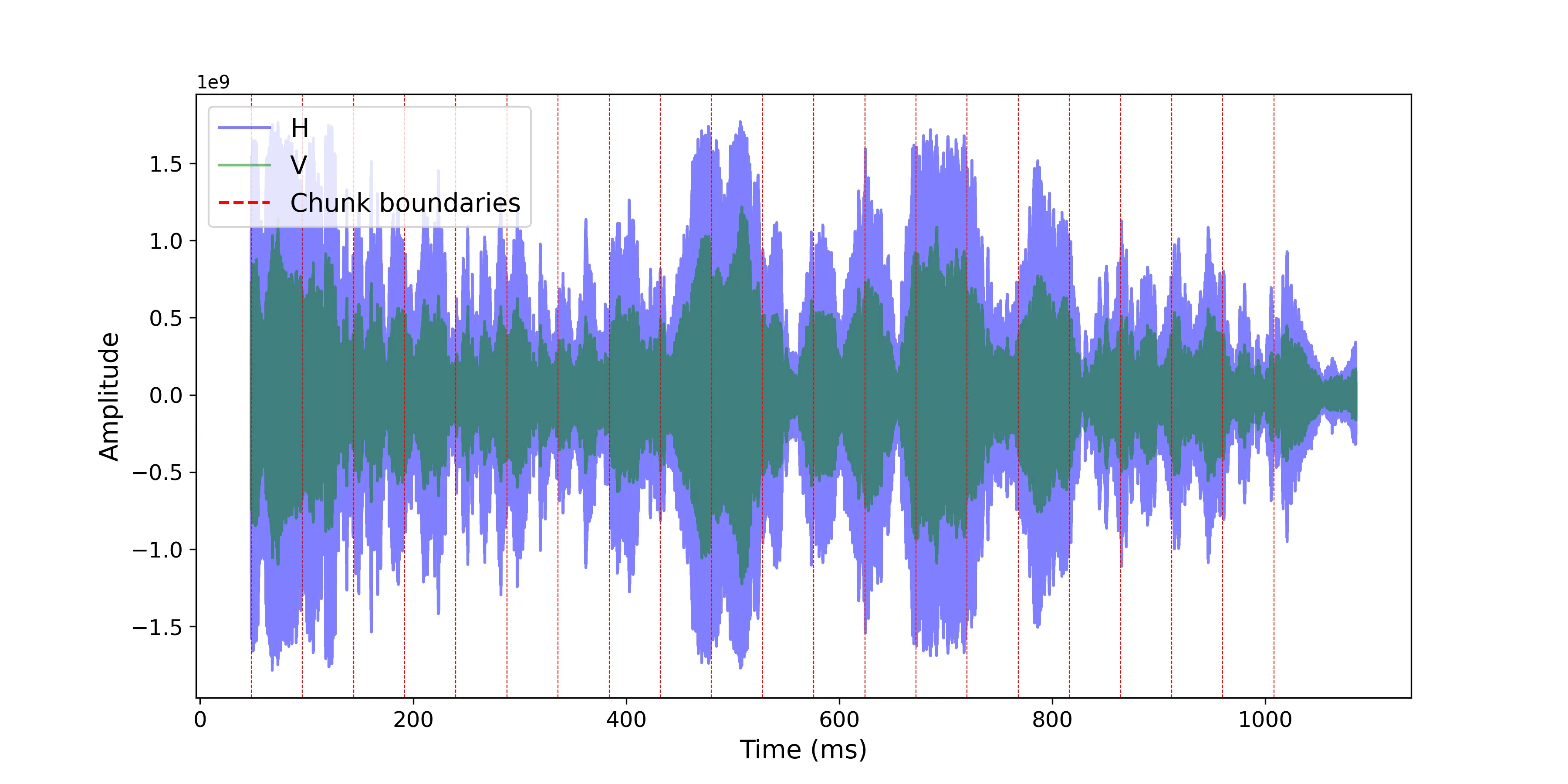
Flat momentum ramp, still H plane

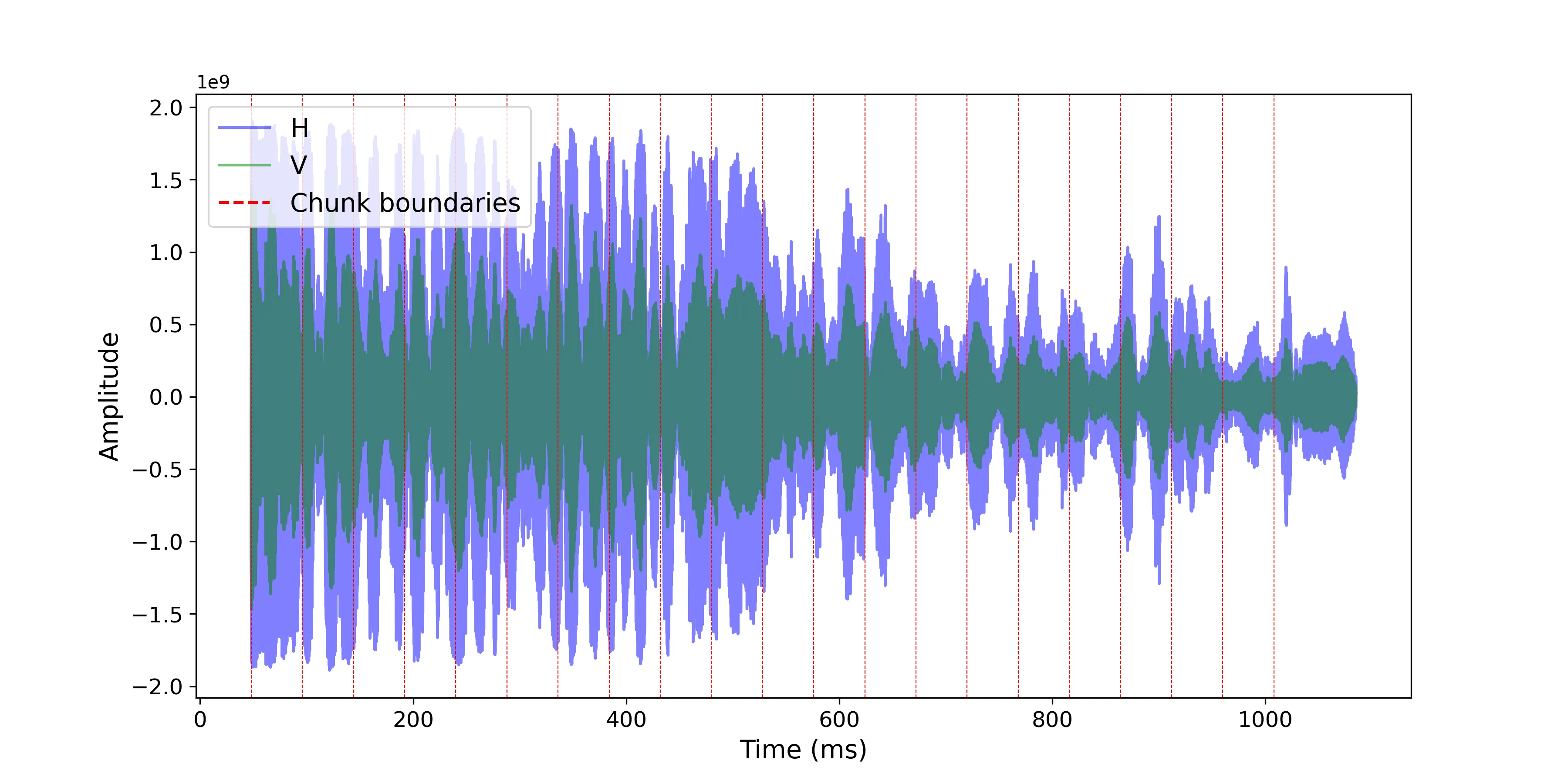
Momentum ramp, V plane

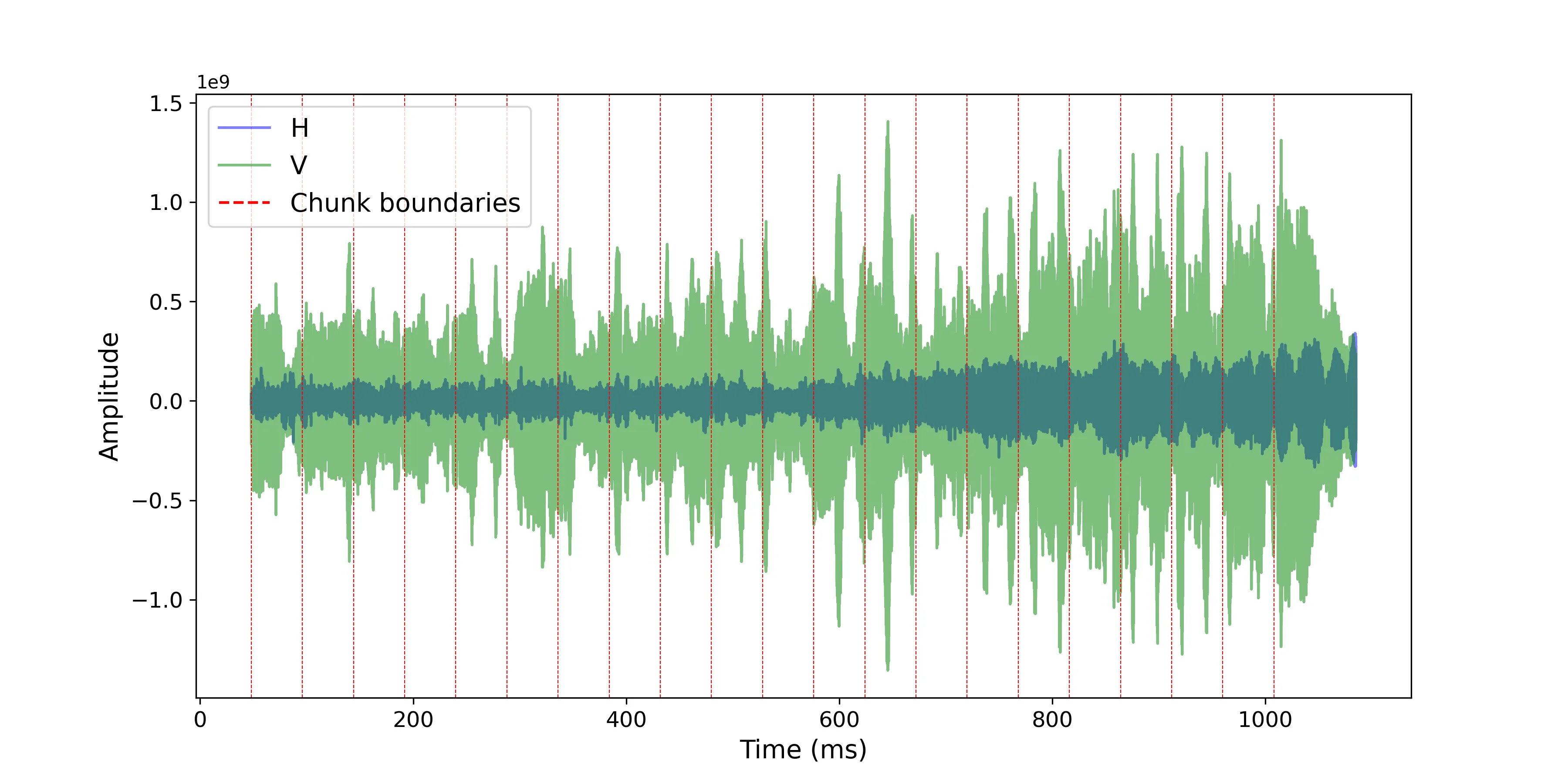
Flat momentum ramp, V plane. The V plane is not excited. 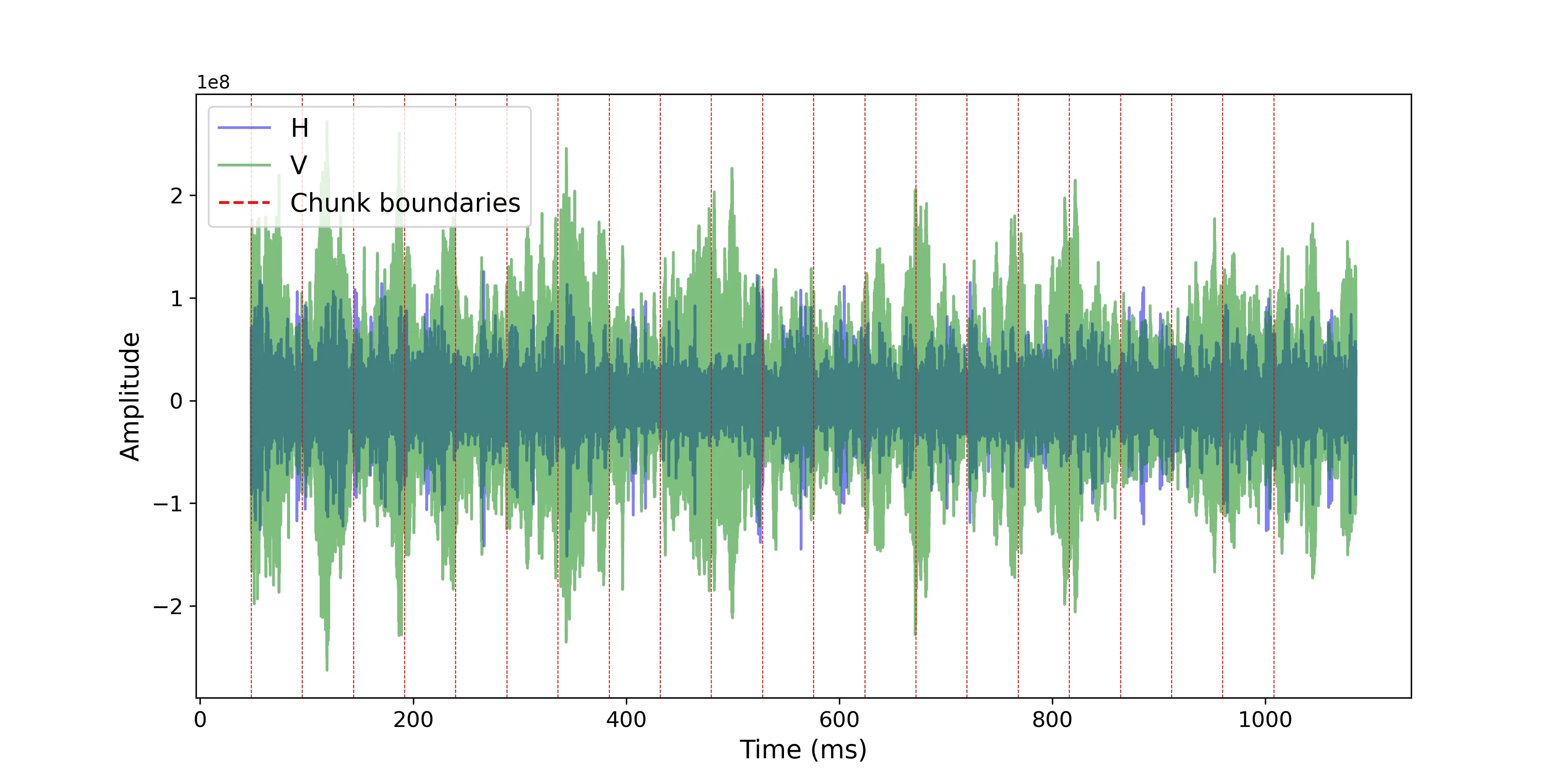The measured tunes are the following, in H and V planes.

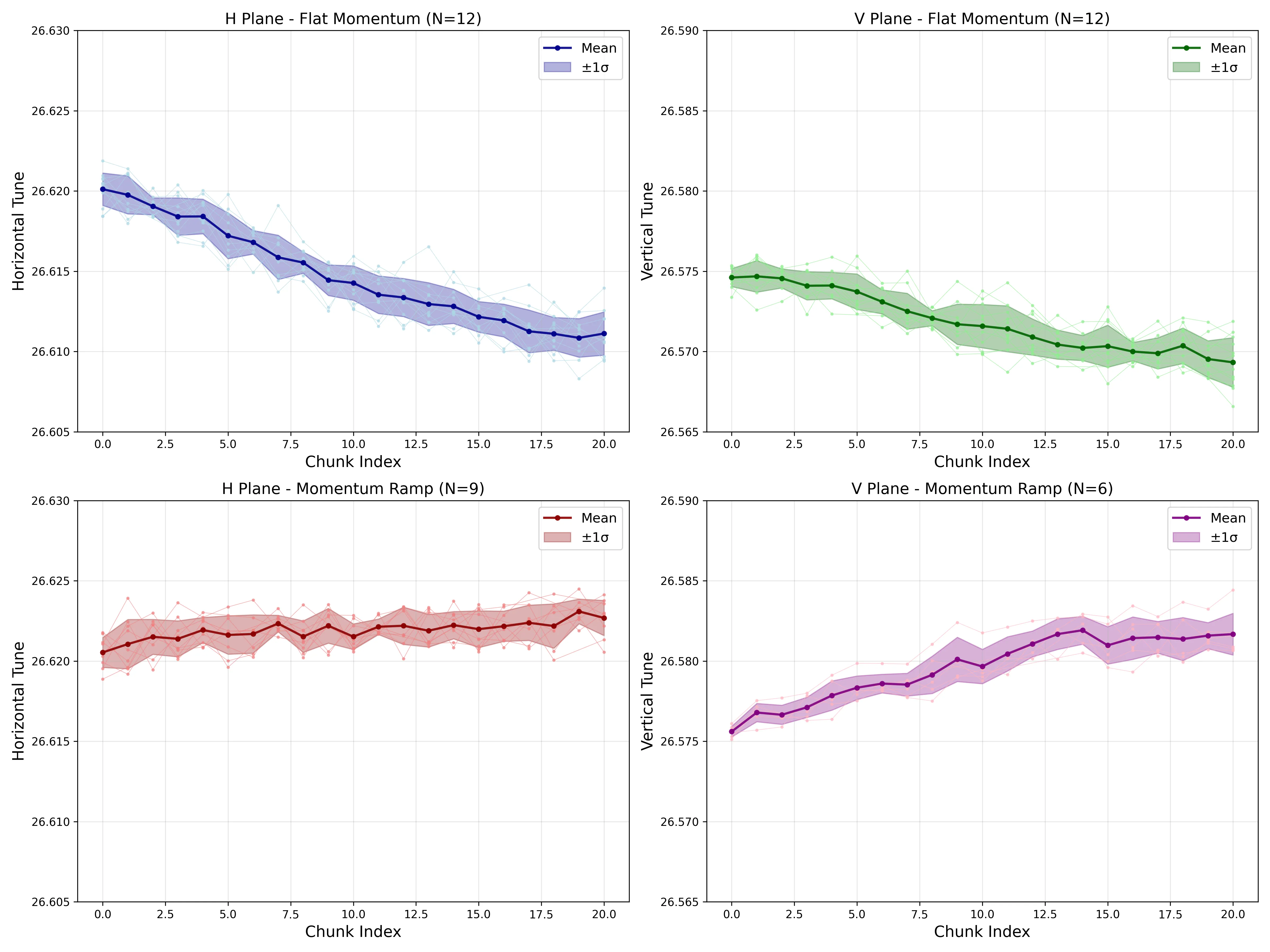
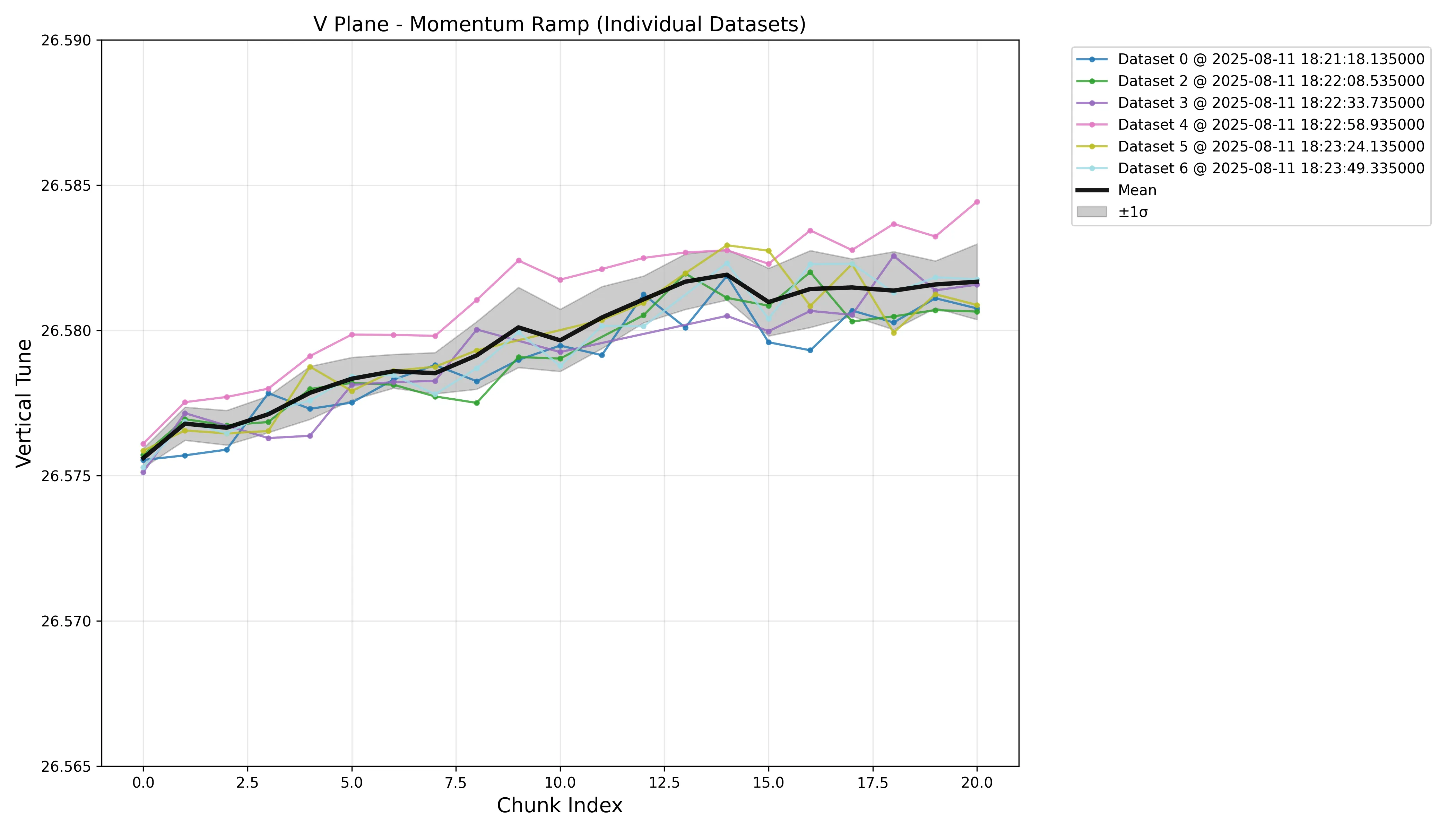
We plot the tunes in the V plane without a momentum ramp, and select only the ones that have initial tune around 0.575, since there seems to be another peak around 0.582, which is wrong. So we lose about half the data. In this case the beam is not excited so the signal is indeed weaker.

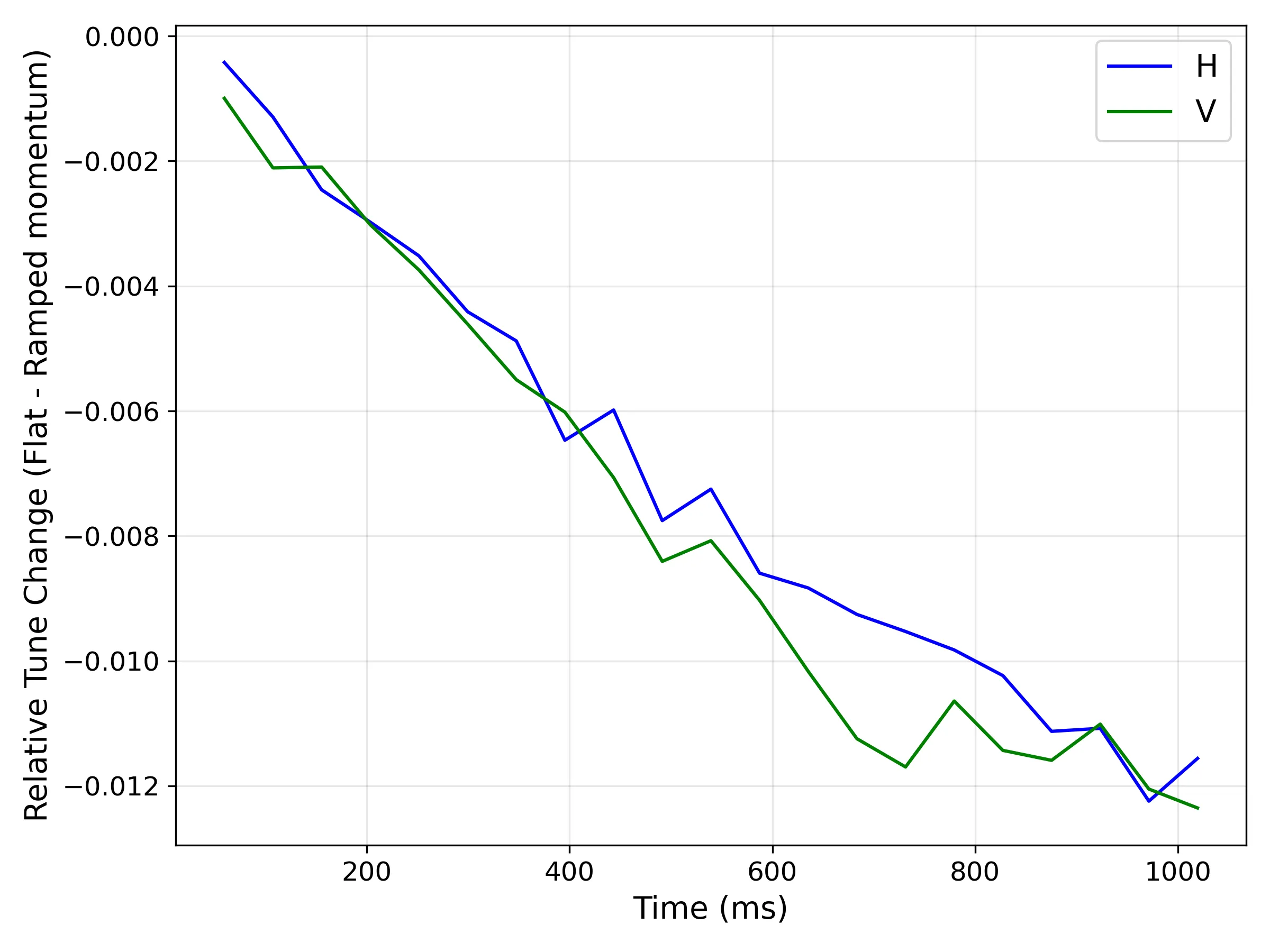
Taking the measured tunes in H and V planes with and without a momentum ramp, we take the pointwise difference to show the relative tune change.

We fit exponentials with 1, 2 or 3 components using scipy.optimize.minimize and perform a joint optimization, fitting both curves with the same time constants, since they should have the same underlying dynamics.

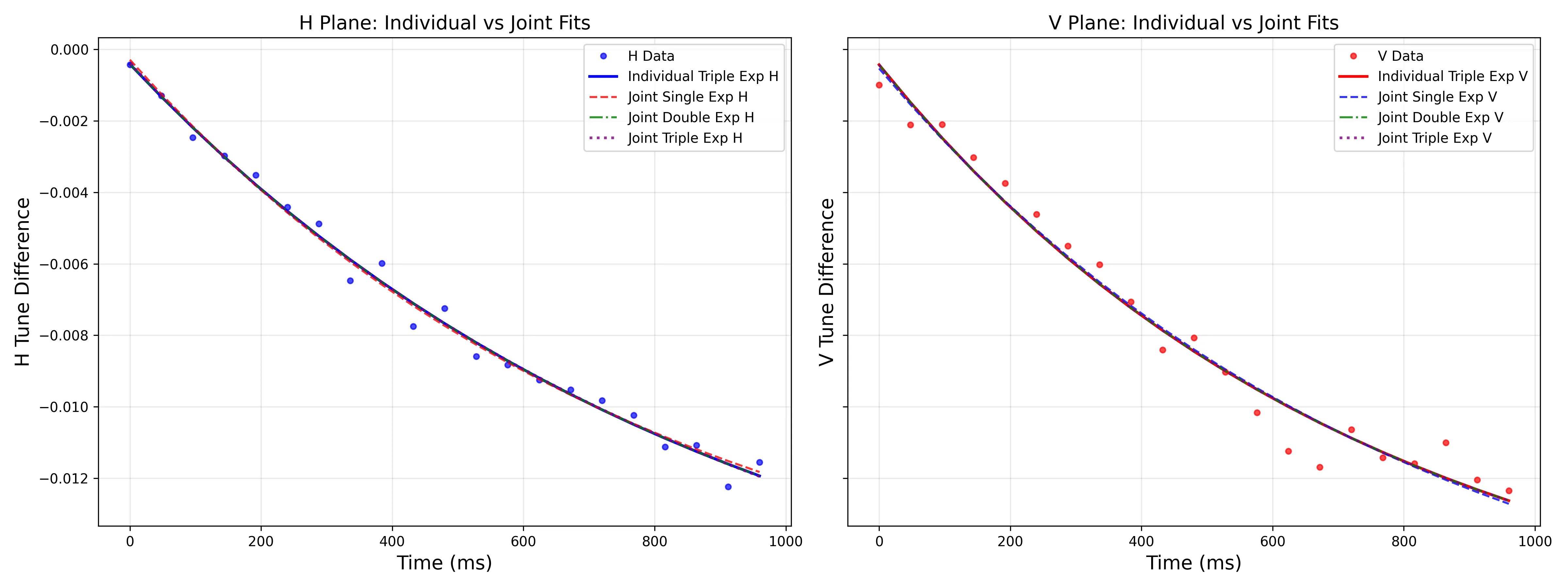
The fits show reveal the following time constants:

Plane	Fit Type	Model	RMSE ($\times 10^{-4}$)	${\tau }_1$ (s)	${\tau }_2$ (s)	${\tau }_3$ (s)
H	Individual	Single	3.42	0.902	-	-
H	Individual	Double	3.42	0.902	4.664	-
H	Individual	Triple	3.42	0.902	4.665	9.334
V	Individual	Single	5.82	0.736	-	-
V	Individual	Double	5.82	0.736	45.470	-
V	Individual	Triple	5.82	0.736	0.404	271.509
H+V	Joint	Single	4.81	0.801	-	-
H+V	Joint	Double	4.77	0.736	0.902	-
H+V	Joint	Triple	4.78	0.738	15.383	163.082

It seems that the decay follows a main ${\tau }_1\approx 800$ ms with a single exponential, and ${\tau }_1\approx 736$ ms and ${\tau }_2\approx 900mswithtwoexponentials.Thetripleexponentialdoesnotfitwell.BasedonthefitRMSE,thedoubleexponentialdoesnotsignificantlyimprovethefit,andwiththelimitednumberofpoints,itwouldsuggestasingleexponentialwith$\tau_1\approx 800$ ms decay, which does not match what is measured on the reference quadrupole, with 2-3x larger time constant.